Section 4.3 — Interpreting linear models¶

This notebook contains the code examples from Section 4.3 Interpreting linear models from the No Bullshit Guide to Statistics.

Notebook setup¶

In [1]:

# Ensure required Python modules are installed
%pip install --quiet numpy scipy seaborn pandas statsmodels ministats

# Ensure required Python modules are installed %pip install --quiet numpy scipy seaborn pandas statsmodels ministats

Note: you may need to restart the kernel to use updated packages.

In [2]:

# load Python modules
import os
import numpy as np
import pandas as pd
import seaborn as sns
import matplotlib.pyplot as plt

# load Python modules import os import numpy as np import pandas as pd import seaborn as sns import matplotlib.pyplot as plt

In [3]:

import statsmodels.formula.api as smf
import statsmodels.api as sm
import statsmodels.stats.api as sms

import statsmodels.formula.api as smf import statsmodels.api as sm import statsmodels.stats.api as sms

In [4]:

# Figures setup
plt.clf()  # needed otherwise `sns.set_theme` doesn't work
sns.set_theme(
    context="paper",
    style="whitegrid",
    palette="colorblind",
    rc={"font.family": "serif",
        "font.serif": ["Palatino", "DejaVu Serif", "serif"],
        "figure.figsize": (5, 3)},
)
%config InlineBackend.figure_format = "retina"

# Figures setup plt.clf() # needed otherwise `sns.set_theme` doesn't work sns.set_theme( context="paper", style="whitegrid", palette="colorblind", rc={"font.family": "serif", "font.serif": ["Palatino", "DejaVu Serif", "serif"], "figure.figsize": (5, 3)}, ) %config InlineBackend.figure_format = "retina"

<Figure size 640x480 with 0 Axes>

In [5]:

# Simple float __repr__  
if int(np.__version__.split(".")[0]) >= 2:
    np.set_printoptions(legacy='1.25')

# set random seed for repeatability
np.random.seed(42)

# Simple float __repr__ if int(np.__version__.split(".")[0]) >= 2: np.set_printoptions(legacy='1.25') # set random seed for repeatability np.random.seed(42)

In [6]:

# Download datasets/ directory if necessary
from ministats import ensure_datasets
ensure_datasets()

# Download datasets/ directory if necessary from ministats import ensure_datasets ensure_datasets()

datasets/ directory present and ready.

Introduction¶

In [7]:

# load the dataset
doctors = pd.read_csv("datasets/doctors.csv")
n = doctors.shape[0]

# fit the model
formula = "score ~ 1 + alc + weed + exrc"
lm2 = smf.ols(formula, data=doctors).fit()

# model degrees of freedom (number of predictors)
p = lm2.df_model

# display the summary table
lm2.summary()

# load the dataset doctors = pd.read_csv("datasets/doctors.csv") n = doctors.shape[0] # fit the model formula = "score ~ 1 + alc + weed + exrc" lm2 = smf.ols(formula, data=doctors).fit() # model degrees of freedom (number of predictors) p = lm2.df_model # display the summary table lm2.summary()

Out[7]:

OLS Regression Results

Dep. Variable:	score	R-squared:	0.842
Model:	OLS	Adj. R-squared:	0.839
Method:	Least Squares	F-statistic:	270.3
Date:	Thu, 27 Nov 2025	Prob (F-statistic):	1.05e-60
Time:	09:25:01	Log-Likelihood:	-547.63
No. Observations:	156	AIC:	1103.
Df Residuals:	152	BIC:	1115.
Df Model:	3
Covariance Type:	nonrobust

	coef	std err	t	P>|t|	[0.025	0.975]
Intercept	60.4529	1.289	46.885	0.000	57.905	63.000
alc	-1.8001	0.070	-25.726	0.000	-1.938	-1.662
weed	-1.0216	0.476	-2.145	0.034	-1.962	-0.081
exrc	1.7683	0.138	12.809	0.000	1.496	2.041

Omnibus:	1.140	Durbin-Watson:	1.828
Prob(Omnibus):	0.565	Jarque-Bera (JB):	0.900
Skew:	0.182	Prob(JB):	0.638
Kurtosis:	3.075	Cond. No.	31.2

Notes:
[1] Standard Errors assume that the covariance matrix of the errors is correctly specified.

Model fit metrics¶

Coefficient of determination¶

In [8]:

lm2.rsquared

lm2.rsquared

Out[8]:

0.8421649167873537

In [9]:

# ALT.
1 - lm2.ssr/lm2.centered_tss

# ALT. 1 - lm2.ssr/lm2.centered_tss

Out[9]:

0.8421649167873537

Adjusted coefficient of determination¶

In [10]:

lm2.rsquared_adj

lm2.rsquared_adj

Out[10]:

0.8390497506713147

In [11]:

# ALT.
1 - (lm2.ssr/(n-p-1)) / (lm2.centered_tss/(n-1))

# ALT. 1 - (lm2.ssr/(n-p-1)) / (lm2.centered_tss/(n-1))

Out[11]:

0.8390497506713147

F-statistic and associated p-value¶

In [12]:

lm2.fvalue, lm2.f_pvalue

lm2.fvalue, lm2.f_pvalue

Out[12]:

(270.3435018926584, 1.0512133413866624e-60)

Log-likelihood¶

In [13]:

lm2.llf

lm2.llf

Out[13]:

-547.6259042117637

In [14]:

# ALT.
from scipy.stats import norm
sigmahat = np.sqrt(lm2.scale)
np.sum(np.log(norm.pdf(lm2.resid,scale=sigmahat)))
# Q: Why not exactly the same as lm2.llf?

# ALT. from scipy.stats import norm sigmahat = np.sqrt(lm2.scale) np.sum(np.log(norm.pdf(lm2.resid,scale=sigmahat))) # Q: Why not exactly the same as lm2.llf?

Out[14]:

-547.651992151218

In [15]:

# How lm2.llf is computed:
SSR = np.sum(lm2.resid**2)
nobs2 = n/2.0
llf = -np.log(SSR)*nobs2                # concentrated likelihood
llf -= ( 1+np.log(np.pi/nobs2) )*nobs2  # with likelihood constant
llf

# How lm2.llf is computed: SSR = np.sum(lm2.resid**2) nobs2 = n/2.0 llf = -np.log(SSR)*nobs2 # concentrated likelihood llf -= ( 1+np.log(np.pi/nobs2) )*nobs2 # with likelihood constant llf

Out[15]:

-547.6259042117637

Information criteria¶

In [16]:

lm2.aic, lm2.bic

lm2.aic, lm2.bic

Out[16]:

(1103.2518084235273, 1115.4512324525256)

In [17]:

# ALT.
2*(p+1) - 2*lm2.llf,  np.log(n)*(p+1) - 2*lm2.llf

# ALT. 2*(p+1) - 2*lm2.llf, np.log(n)*(p+1) - 2*lm2.llf

Out[17]:

(1103.2518084235273, 1115.4512324525256)

Other model-fit metrics¶

The mean squared error (MSE)

In [18]:

from statsmodels.tools.eval_measures import mse

scores = doctors["score"]
scorehats = lm2.fittedvalues
mse(scores,scorehats), lm2.ssr/n

from statsmodels.tools.eval_measures import mse scores = doctors["score"] scorehats = lm2.fittedvalues mse(scores,scorehats), lm2.ssr/n

Out[18]:

(65.56013803717556, 65.56013803717556)

Parameter estimates¶

In [19]:

# estimated parameters
lm2.params

# estimated parameters lm2.params

Out[19]:

Intercept    60.452901
alc          -1.800101
weed         -1.021552
exrc          1.768289
dtype: float64

In [20]:

# estimated sigma (std. of error term)
sigmahat = np.sqrt(lm2.scale)
sigmahat

# estimated sigma (std. of error term) sigmahat = np.sqrt(lm2.scale) sigmahat

Out[20]:

8.20276811982562

In [21]:

# ALT.
np.sqrt(lm2.ssr/(n-p-1))

# ALT. np.sqrt(lm2.ssr/(n-p-1))

Out[21]:

8.20276811982562

Confidence intervals for model parameters¶

In [22]:

# standard errors
lm2.bse

# standard errors lm2.bse

Out[22]:

Intercept    1.289380
alc          0.069973
weed         0.476166
exrc         0.138056
dtype: float64

In [23]:

lm2.conf_int(alpha=0.05)

lm2.conf_int(alpha=0.05)

Out[23]:

	0	1
Intercept	57.905480	63.000321
alc	-1.938347	-1.661856
weed	-1.962309	-0.080794
exrc	1.495533	2.041044

Hypothesis testing for linear models¶

T-tests for individual parameters¶

Hypothesis testing for slope coefficient

Is there a non-zero slope coefficient?

Example: t-test for the variable weed¶

• Null hypothesis $H_0$: weed has no effect on score, which is equivalent to $\beta_{\texttt{weed}} = 0$:

  $$ H_0: \quad S \;\sim\; \mathcal{N}( {\color{red} \beta_0 + \beta_{\texttt{alc}}\!\cdot\!\textrm{alc} + \beta_{\texttt{exrc}}\!\cdot\!\textrm{exrc} }, \ \sigma) \qquad \qquad $$

• Alternative hypothesis $H_A$: weed has an effect on score, and the slope is not zero, $\beta_{\texttt{weed}} \neq 0$:

  $$ H_A: \quad S \;\sim\; \mathcal{N}\left( {\color{blue} \beta_0 + \beta_{\texttt{alc}}\!\cdot\!\textrm{alc} + \beta_{\texttt{weed}}\!\cdot\!\textrm{weed} + \beta_{\texttt{exrc}}\!\cdot\!\textrm{exrc} }, \ \sigma \right) $$

In [24]:

lm2.tvalues["weed"], lm2.pvalues["weed"], n-p-1

lm2.tvalues["weed"], lm2.pvalues["weed"], n-p-1

Out[24]:

(-2.1453705454368617, 0.03351156181342317, 152.0)

Calculate the $t$ statistic:

In [25]:

obst_weed = (lm2.params["weed"] - 0) / lm2.bse["weed"]
obst_weed  # = lm2.tvalues["weed"]

obst_weed = (lm2.params["weed"] - 0) / lm2.bse["weed"] obst_weed # = lm2.tvalues["weed"]

Out[25]:

-2.1453705454368617

Calculate the associated $p$-value

In [26]:

from scipy.stats import t as tdist

pleft = tdist(df=n-p-1).cdf(obst_weed)
pright = 1 - tdist(df=lm2.df_resid).cdf(obst_weed)
pvalue_weed = 2 * min(pleft, pright)
pvalue_weed  # = lm2.pvalues["weed"]

from scipy.stats import t as tdist pleft = tdist(df=n-p-1).cdf(obst_weed) pright = 1 - tdist(df=lm2.df_resid).cdf(obst_weed) pvalue_weed = 2 * min(pleft, pright) pvalue_weed # = lm2.pvalues["weed"]

Out[26]:

0.03351156181342317

In [27]:

lm2.tvalues

lm2.tvalues

Out[27]:

Intercept    46.885245
alc         -25.725654
weed         -2.145371
exrc         12.808529
dtype: float64

In [28]:

lm2.df_resid, n-p-1

lm2.df_resid, n-p-1

Out[28]:

(152.0, 152.0)

In [29]:

lm2.pvalues

lm2.pvalues

Out[29]:

Intercept    2.756807e-92
alc          2.985013e-57
weed         3.351156e-02
exrc         6.136296e-26
dtype: float64

F-test for the overall model¶

In [30]:

lm2.fvalue

lm2.fvalue

Out[30]:

270.3435018926584

In [31]:

# ALT.
F = lm2.mse_model / lm2.mse_resid
F

# ALT. F = lm2.mse_model / lm2.mse_resid F

Out[31]:

270.3435018926584

In [32]:

lm2.f_pvalue

lm2.f_pvalue

Out[32]:

1.0512133413866624e-60

In [33]:

# ALT.
from scipy.stats import f as fdist
fdist(dfn=p, dfd=n-p-1).sf(F)

# ALT. from scipy.stats import f as fdist fdist(dfn=p, dfd=n-p-1).sf(F)

Out[33]:

1.0512133413866624e-60

F-test for a submodel¶

In [34]:

formula2nw = "score ~ 1 + alc + exrc"
lm2_noweed = smf.ols(formula2nw, data=doctors).fit()
F_noweed, p_noweed, _ = lm2.compare_f_test(lm2_noweed)
F_noweed, p_noweed

formula2nw = "score ~ 1 + alc + exrc" lm2_noweed = smf.ols(formula2nw, data=doctors).fit() F_noweed, p_noweed, _ = lm2.compare_f_test(lm2_noweed) F_noweed, p_noweed

Out[34]:

(4.602614777228041, 0.03351156181342345)

The F-statistic is the same as the t-statistic¶

In [35]:

F_noweed, obst_weed**2, lm2.tvalues["weed"]**2

F_noweed, obst_weed**2, lm2.tvalues["weed"]**2

Out[35]:

(4.602614777228041, 4.602614777228057, 4.602614777228057)

In [36]:

p_noweed, pvalue_weed, lm2.pvalues["weed"]

p_noweed, pvalue_weed, lm2.pvalues["weed"]

Out[36]:

(0.03351156181342345, 0.03351156181342317, 0.03351156181342317)

Assumptions checks and diagnostics¶

Are the assumptions for the linear model satisfied?

Residuals plots¶

In [37]:

from ministats import plot_resid
plot_resid(lm2, lowess=True);

from ministats import plot_resid plot_resid(lm2, lowess=True);

In [38]:

from ministats import plot_resid
plot_resid(lm2, pred="alc", lowess=True);

from ministats import plot_resid plot_resid(lm2, pred="alc", lowess=True);

Linearity checks¶

Look at residuals plots.

Independence checks¶

Look at residuals plots.

Normality checks¶

Look at residuals plots...

QQ plot inspection¶

In [39]:

from statsmodels.graphics.api import qqplot
qqplot(lm2.resid, line="s");

from statsmodels.graphics.api import qqplot qqplot(lm2.resid, line="s");

In [40]:

# BONUS
ax = sns.histplot(lm2.resid)
ax.set_xlim([-27,27]);

# BONUS ax = sns.histplot(lm2.resid) ax.set_xlim([-27,27]);

Skew and kurtosis¶

In [41]:

from scipy.stats import skew
from scipy.stats import kurtosis

skew(lm2.resid), kurtosis(lm2.resid, fisher=False)

from scipy.stats import skew from scipy.stats import kurtosis skew(lm2.resid), kurtosis(lm2.resid, fisher=False)

Out[41]:

(0.18224568453683537, 3.0747952385562645)

Homoscedasticity checks¶

The scale-location plot allows us to see if pattern in the variance of the residuals exists.

In [42]:

from ministats import plot_scaleloc

plot_scaleloc(lm2);

from ministats import plot_scaleloc plot_scaleloc(lm2);

In [43]:

# ALT. Generate the scale-location plot from scratch

# 1. Compute the square root of the standardized residuals
scorehats = lm2.fittedvalues
std_resids = lm2.resid / np.sqrt(lm2.scale)
sqrt_std_resids = np.sqrt(np.abs(std_resids))

# 2. Generate the scatter plot
ax = sns.scatterplot(x=scorehats, y=sqrt_std_resids)

# 3. Add the LOWESS curve
from statsmodels.nonparametric.smoothers_lowess import lowess
xgrid, ylowess = lowess(sqrt_std_resids, scorehats).T
sns.lineplot(x=xgrid, y=ylowess, ax=ax)

# 4. Add descriptive labels
ax.set_ylabel(r"$\sqrt{|standardized\ residuals|}$")
ax.set_xlabel("fitted values");

# ALT. Generate the scale-location plot from scratch # 1. Compute the square root of the standardized residuals scorehats = lm2.fittedvalues std_resids = lm2.resid / np.sqrt(lm2.scale) sqrt_std_resids = np.sqrt(np.abs(std_resids)) # 2. Generate the scatter plot ax = sns.scatterplot(x=scorehats, y=sqrt_std_resids) # 3. Add the LOWESS curve from statsmodels.nonparametric.smoothers_lowess import lowess xgrid, ylowess = lowess(sqrt_std_resids, scorehats).T sns.lineplot(x=xgrid, y=ylowess, ax=ax) # 4. Add descriptive labels ax.set_ylabel(r"$\sqrt{|standardized\ residuals|}$") ax.set_xlabel("fitted values");

Collinearity checks¶

Check the correlation matrix¶

In [44]:

corrM = doctors[["alc", "weed", "exrc"]].corr()
corrM.round(4)

corrM = doctors[["alc", "weed", "exrc"]].corr() corrM.round(4)

Out[44]:

	alc	weed	exrc
alc	1.0000	0.0422	0.0336
weed	0.0422	1.0000	0.0952
exrc	0.0336	0.0952	1.0000

In [45]:

# # BONUS 1 (not covered anywhere earlier in the book)
# sns.heatmap(corrM, annot=True, fmt='.2f', cmap="Grays");

# # BONUS 1 (not covered anywhere earlier in the book) # sns.heatmap(corrM, annot=True, fmt='.2f', cmap="Grays");

In [46]:

# # BONUS 2 (not covered anywhere earlier in the book)
# sns.pairplot(doctors[["alc", "weed", "exrc"]]);

# # BONUS 2 (not covered anywhere earlier in the book) # sns.pairplot(doctors[["alc", "weed", "exrc"]]);

Condition number¶

In [47]:

lm2.condition_number

lm2.condition_number

Out[47]:

31.229721453770157

In [48]:

# ALT. (compute from scratch)
#######################################################
X = sm.add_constant(doctors[["alc","weed","exrc"]])
eigvals = np.linalg.eigvals(X.T @ X)
lam_max, lam_min = np.max(eigvals), np.min(eigvals)
np.sqrt(lam_max/lam_min)

# ALT. (compute from scratch) ####################################################### X = sm.add_constant(doctors[["alc","weed","exrc"]]) eigvals = np.linalg.eigvals(X.T @ X) lam_max, lam_min = np.max(eigvals), np.min(eigvals) np.sqrt(lam_max/lam_min)

Out[48]:

31.22972145377028

Variance inflation factor¶

In [49]:

from ministats import calc_lm_vif

calc_lm_vif(lm2, "alc"), calc_lm_vif(lm2, "weed"), calc_lm_vif(lm2, "exrc")

from ministats import calc_lm_vif calc_lm_vif(lm2, "alc"), calc_lm_vif(lm2, "weed"), calc_lm_vif(lm2, "exrc")

Out[49]:

(1.002669215630476, 1.0107031450073227, 1.010048809433661)

In [50]:

# ALT. using variance_inflation_factor from statsmodels
from statsmodels.stats.outliers_influence \
     import variance_inflation_factor as statsmodels_vif

X = sm.add_constant(doctors[["alc","weed","exrc"]])
statsmodels_vif(X, 1)  # variation inflation factor of "alc" in lm2

# ALT. using variance_inflation_factor from statsmodels from statsmodels.stats.outliers_influence \ import variance_inflation_factor as statsmodels_vif X = sm.add_constant(doctors[["alc","weed","exrc"]]) statsmodels_vif(X, 1) # variation inflation factor of "alc" in lm2

Out[50]:

1.002669215630476

Perfect multicollinearity example¶

In [51]:

doctorscol = doctors.copy()
doctorscol["alc2"] = doctors["alc"]
formula2col = "score ~ 1 + alc + alc2 + weed + exrc"
lm2col = smf.ols(formula2col, data=doctorscol).fit()
lm2col.params

doctorscol = doctors.copy() doctorscol["alc2"] = doctors["alc"] formula2col = "score ~ 1 + alc + alc2 + weed + exrc" lm2col = smf.ols(formula2col, data=doctorscol).fit() lm2col.params

Out[51]:

Intercept    60.452901
alc          -0.900051
alc2         -0.900051
weed         -1.021552
exrc          1.768289
dtype: float64

In [52]:

calc_lm_vif(lm2col, "alc")

calc_lm_vif(lm2col, "alc")

/Users/ivan/Projects/Minireference/software/ministats/ministats/linear_models.py:17: RuntimeWarning: divide by zero encountered in scalar divide
  vif = 1. / (1. - r_squared_i)

Out[52]:

inf

Outliers and influential observations¶

TODO: definitions

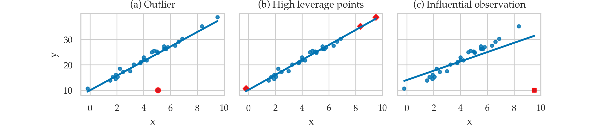
Leverage and influence metrics¶

TODO: add definitions of quantities in point form

Leverage plots¶

In [53]:

from statsmodels.graphics.api import plot_leverage_resid2

plot_leverage_resid2(lm2);

from statsmodels.graphics.api import plot_leverage_resid2 plot_leverage_resid2(lm2);

Influence plots¶

In [54]:

from statsmodels.graphics.api import influence_plot

influence_plot(lm2, criterion="cooks", size=4);

from statsmodels.graphics.api import influence_plot influence_plot(lm2, criterion="cooks", size=4);

Model predictions¶

Prediction on the dataset¶

In [55]:

lm2.fittedvalues

lm2.fittedvalues

Out[55]:

0      55.345142
1      32.408174
2      71.030821
3      56.789073
4      57.514154
         ...    
151    58.867105
152    43.049719
153    57.728460
154    69.617361
155    78.135788
Length: 156, dtype: float64

Prediction for new data¶

In [56]:

newdoc = {"alc":3, "weed":1, "exrc":8}
lm2.predict(newdoc)

newdoc = {"alc":3, "weed":1, "exrc":8} lm2.predict(newdoc)

Out[56]:

0    68.177355
dtype: float64

In [57]:

newdoc_score_pred = lm2.get_prediction(newdoc)
newdoc_score_pred.conf_int(obs=True, alpha=0.1)

newdoc_score_pred = lm2.get_prediction(newdoc) newdoc_score_pred.conf_int(obs=True, alpha=0.1)

Out[57]:

array([[54.50324518, 81.85146489]])

In-sample prediction accuracy¶

In [58]:

# Compute the in-sample mean squared error (MSE)
scores = doctors['score']
scorehats = lm2.fittedvalues
mse = np.mean( (scores - scorehats)**2 )
mse

# Compute the in-sample mean squared error (MSE) scores = doctors['score'] scorehats = lm2.fittedvalues mse = np.mean( (scores - scorehats)**2 ) mse

Out[58]:

65.56013803717556

In [59]:

# ALT.
lm2.ssr/n

# ALT. lm2.ssr/n

Out[59]:

65.56013803717556

In [60]:

# # ALT2.
# from statsmodels.tools.eval_measures import mse
# mse(scores,scorehats)

# # ALT2. # from statsmodels.tools.eval_measures import mse # mse(scores,scorehats)

Out-of-sample prediction accuracy¶

TODO: explain

Leave-one-out cross-validation¶

In [61]:

loo_preds = np.zeros(n)
for i in range(n):
    doctors_no_i = doctors.drop(index=i)
    lm2_no_i = smf.ols(formula,data=doctors_no_i).fit()
    predictors_i = dict(doctors.loc[i,:])
    pred_i = lm2_no_i.predict(predictors_i)[0]
    loo_preds[i] = pred_i

# Calculate the out-of-sample mean squared error
mse_loo = np.mean( (doctors['score'] - loo_preds)**2 )
mse_loo

loo_preds = np.zeros(n) for i in range(n): doctors_no_i = doctors.drop(index=i) lm2_no_i = smf.ols(formula,data=doctors_no_i).fit() predictors_i = dict(doctors.loc[i,:]) pred_i = lm2_no_i.predict(predictors_i)[0] loo_preds[i] = pred_i # Calculate the out-of-sample mean squared error mse_loo = np.mean( (doctors['score'] - loo_preds)**2 ) mse_loo

Out[61]:

69.20054514710952

Compare with the in-sample MSE of the model which is lower.

In [62]:

lm2.ssr/n

lm2.ssr/n

Out[62]:

65.56013803717556

Towards machine learning¶

The out-of-sample prediction accuracy is a common metric used in machine learning (ML) tasks.

Explanations¶

Adjusted $R^2$¶

TODO: show formula

In [63]:

# TODO 

# TODO

Calculating standard error of parameters (optional)¶

In [64]:

lm2.bse

lm2.bse

Out[64]:

Intercept    1.289380
alc          0.069973
weed         0.476166
exrc         0.138056
dtype: float64

In [65]:

# construct the design matrix for the model 
X = sm.add_constant(doctors[["alc","weed","exrc"]])
# calculate the diagonal of the inverse-covariance matrix
inv_covs = np.diag(np.linalg.inv(X.T.dot(X)))
sigmahat*np.sqrt(inv_covs)

# construct the design matrix for the model X = sm.add_constant(doctors[["alc","weed","exrc"]]) # calculate the diagonal of the inverse-covariance matrix inv_covs = np.diag(np.linalg.inv(X.T.dot(X))) sigmahat*np.sqrt(inv_covs)

Out[65]:

array([1.28938008, 0.06997301, 0.4761656 , 0.13805557])

In [66]:

# these lead to approx. same result because predictors are not correlated
# but the correct formula is to use the inv. covariance matrix as above.
sum_alc_dev2 = np.sum((doctors["alc"] - doctors["alc"].mean())**2)
sum_weed_dev2 = np.sum((doctors["weed"] - doctors["weed"].mean())**2)
sum_exrc_dev2 = np.sum((doctors["exrc"] - doctors["exrc"].mean())**2)
se_b_alc = sigmahat / np.sqrt(sum_alc_dev2)
se_b_weed = sigmahat / np.sqrt(sum_weed_dev2)
se_b_exrc = sigmahat / np.sqrt(sum_exrc_dev2)
se_b_alc, se_b_weed, se_b_exrc

# these lead to approx. same result because predictors are not correlated # but the correct formula is to use the inv. covariance matrix as above. sum_alc_dev2 = np.sum((doctors["alc"] - doctors["alc"].mean())**2) sum_weed_dev2 = np.sum((doctors["weed"] - doctors["weed"].mean())**2) sum_exrc_dev2 = np.sum((doctors["exrc"] - doctors["exrc"].mean())**2) se_b_alc = sigmahat / np.sqrt(sum_alc_dev2) se_b_weed = sigmahat / np.sqrt(sum_weed_dev2) se_b_exrc = sigmahat / np.sqrt(sum_exrc_dev2) se_b_alc, se_b_weed, se_b_exrc

Out[66]:

(0.06987980522527786, 0.4736376432238542, 0.1373671047363984)

Metrics for influential observations¶

Leverage score¶

$$ h_i = 1 - \frac{r_i}{r_{i(i)}}, $$

In [67]:

infl = lm2.get_influence()
infl.hat_matrix_diag[0:5]

infl = lm2.get_influence() infl.hat_matrix_diag[0:5]

Out[67]:

array([0.09502413, 0.0129673 , 0.01709783, 0.01465484, 0.00981632])

Studentized residuals¶

$$ t_{i} = \frac{r_i}{\hat{\sigma}_{(i)} \sqrt{1-h_i}} $$

In [68]:

infl.resid_studentized_external[0:5]

infl.resid_studentized_external[0:5]

Out[68]:

array([ 0.98085317, -2.03409243, -1.61072775, -0.21903275, -1.29094028])

Cook's distance¶

$$ D_i = \frac{r_i^2}{p \, \widehat{\sigma}^2} \cdot \frac{h_{i}}{(1-h_{i})^2} % = \frac{t_i^2 }{p}\frac{h_i}{1-h_i} $$

In [69]:

infl.cooks_distance[0][0:5]

infl.cooks_distance[0][0:5]

Out[69]:

array([0.02526116, 0.01331454, 0.01116562, 0.00017951, 0.0041123 ])

DFFITS diagnostic¶

$$ \textrm{DFFITS}_i = \frac{ \widehat{y}_i - \widehat{y}_{i(i)} }{ \widehat{\sigma}_{(i)} \sqrt{h_i} }. $$

In [70]:

infl.dffits[0][0:5]

infl.dffits[0][0:5]

Out[70]:

array([ 0.31783554, -0.23314692, -0.21244055, -0.02671194, -0.12853536])

Calculating leverage and influence metrics using statsmodels¶

In [71]:

infl = lm2.get_influence()
infl_df = infl.summary_frame()
# list(infl_df.columns)

infl = lm2.get_influence() infl_df = infl.summary_frame() # list(infl_df.columns)

In [72]:

cols = ["student_resid", "hat_diag", "cooks_d", "dffits"]
infl_df[cols].round(3).head(5)

cols = ["student_resid", "hat_diag", "cooks_d", "dffits"] infl_df[cols].round(3).head(5)

Out[72]:

	student_resid	hat_diag	cooks_d	dffits
0	0.981	0.095	0.025	0.318
1	-2.034	0.013	0.013	-0.233
2	-1.611	0.017	0.011	-0.212
3	-0.219	0.015	0.000	-0.027
4	-1.291	0.010	0.004	-0.129

Hypothesis tests for checking linear model assumptions¶

In [73]:

lm2.diagn

lm2.diagn

Out[73]:

{'jb': 0.899913857959268,
 'jbpv': 0.6376556155083223,
 'skew': 0.18224568453683537,
 'kurtosis': 3.0747952385562645,
 'omni': 1.1403999852814093,
 'omnipv': 0.5654123490825886,
 'condno': 31.229721453770157,
 'mineigval': 40.14996367643264}

Hypothesis test for linearity¶

In [74]:

sms.linear_harvey_collier(lm2)

sms.linear_harvey_collier(lm2)

Out[74]:

TtestResult(statistic=1.4317316989777142, pvalue=0.15427366179829288, df=152)

Normality tests¶

In [75]:

from statsmodels.stats.stattools import omni_normtest

omni, omnipv = omni_normtest(lm2.resid)
omni, omnipv

from statsmodels.stats.stattools import omni_normtest omni, omnipv = omni_normtest(lm2.resid) omni, omnipv

Out[75]:

(1.1403999852814093, 0.5654123490825886)

In [76]:

from statsmodels.stats.stattools import jarque_bera

jb, jbpv, skew, kurtosis = jarque_bera(lm2.resid)
jb, jbpv, skew, kurtosis

from statsmodels.stats.stattools import jarque_bera jb, jbpv, skew, kurtosis = jarque_bera(lm2.resid) jb, jbpv, skew, kurtosis

Out[76]:

(0.899913857959268,
 0.6376556155083223,
 0.18224568453683537,
 3.0747952385562645)

Independence test (autocorrelation)¶

In [77]:

from statsmodels.stats.stattools import durbin_watson

durbin_watson(lm2.resid)

from statsmodels.stats.stattools import durbin_watson durbin_watson(lm2.resid)

Out[77]:

1.8284830211766738

Homoskedasticity tests¶

Breusch-Pagan¶

https://en.wikipedia.org/wiki/Breusch-Pagan_test

In [78]:

lm, p_lm, _, _ = sms.het_breuschpagan(lm2.resid, lm2.model.exog)
lm, p_lm

lm, p_lm, _, _ = sms.het_breuschpagan(lm2.resid, lm2.model.exog) lm, p_lm

Out[78]:

(6.254809752854332, 0.09985027888796476)

Goldfeld-Quandt test¶

https://en.wikipedia.org/wiki/Goldfeld-Quandt_test

In [79]:

# sort by score
idxs = doctors.sort_values("alc").index

# sort by scorehats
idxs = np.argsort(lm2.fittedvalues)
X = lm2.model.exog[idxs,:]
resid = lm2.resid[idxs]

# run the test
F, p_F, _ = sms.het_goldfeldquandt(resid, X, idx=1)
F, p_F

# sort by score idxs = doctors.sort_values("alc").index # sort by scorehats idxs = np.argsort(lm2.fittedvalues) X = lm2.model.exog[idxs,:] resid = lm2.resid[idxs] # run the test F, p_F, _ = sms.het_goldfeldquandt(resid, X, idx=1) F, p_F

Out[79]:

(1.5346515257083706, 0.03369473000286669)

Discussion¶

Maximum likelihood estimate¶

In [80]:

from scipy.optimize import minimize
from scipy.stats import norm

n = len(doctors)
preds = doctors[["alc", "weed", "exrc"]]
scores = doctors["score"]

def neg_log_likelihood(betas):
    scorehats = betas[0] + (betas[1:]*preds).sum(1)
    residuals = scores - scorehats
    SSR = np.sum(residuals**2)
    sigmahat_MLE = np.sqrt(SSR/n)
    likelihoods = norm.pdf(residuals, scale=sigmahat_MLE)
    log_likelihood = np.sum(np.log(likelihoods))
    return -log_likelihood

betas = minimize(neg_log_likelihood, x0=[0,0,0,0]).x
betas

from scipy.optimize import minimize from scipy.stats import norm n = len(doctors) preds = doctors[["alc", "weed", "exrc"]] scores = doctors["score"] def neg_log_likelihood(betas): scorehats = betas[0] + (betas[1:]*preds).sum(1) residuals = scores - scorehats SSR = np.sum(residuals**2) sigmahat_MLE = np.sqrt(SSR/n) likelihoods = norm.pdf(residuals, scale=sigmahat_MLE) log_likelihood = np.sum(np.log(likelihoods)) return -log_likelihood betas = minimize(neg_log_likelihood, x0=[0,0,0,0]).x betas

Out[80]:

array([60.45288852, -1.80010089, -1.0215511 ,  1.76828937])

In [81]:

# the results are the same as `lm2.params`
lm2.params.values

# the results are the same as `lm2.params` lm2.params.values

Out[81]:

array([60.45290059, -1.80010132, -1.02155166,  1.76828876])

In [82]:

# calculate the maximum log-likelihood achieved
-neg_log_likelihood(betas), lm2.llf

# calculate the maximum log-likelihood achieved -neg_log_likelihood(betas), lm2.llf

Out[82]:

(-547.6259042118089, -547.6259042117637)

Regularization¶

In [83]:

doctors[["alc", "weed", "exrc"]].std()

doctors[["alc", "weed", "exrc"]].std()

Out[83]:

alc     9.428506
weed    1.391068
exrc    4.796361
dtype: float64

In [84]:

# TRUE
# alc =  - 1.8
# weed = - 0.5
# exrc = + 1.9

# FITTED
lm2.params

# TRUE # alc = - 1.8 # weed = - 0.5 # exrc = + 1.9 # FITTED lm2.params

Out[84]:

Intercept    60.452901
alc          -1.800101
weed         -1.021552
exrc          1.768289
dtype: float64

L1 regularization (LASSO)¶

Set alpha option to the desired value $\alpha_1$ and L1_wt = 1, which means $100\%$ L1 regularization.

In [85]:

lm2_L1reg = smf.ols(formula, data=doctors) \
               .fit_regularized(alpha=0.3, L1_wt=1.0)
lm2_L1reg.params

lm2_L1reg = smf.ols(formula, data=doctors) \ .fit_regularized(alpha=0.3, L1_wt=1.0) lm2_L1reg.params

Out[85]:

Intercept    58.930367
alc          -1.763306
weed          0.000000
exrc          1.795228
dtype: float64

L2 regularization (ridge)¶

Set alpha option to the desired value $\alpha_2$ and L1_wt = 0, which means $0\%$ L1 regularization and $100\%$ L2 regularization.

In [86]:

lm2_L2reg = smf.ols(formula, data=doctors) \
               .fit_regularized(alpha=0.05, L1_wt=0.0001)
lm2_L2reg.params

lm2_L2reg = smf.ols(formula, data=doctors) \ .fit_regularized(alpha=0.05, L1_wt=0.0001) lm2_L2reg.params

Out[86]:

Intercept    50.694960
alc          -1.472536
weed         -0.457425
exrc          2.323386
dtype: float64

Statsmodels diagnostics plots (BONUS TOPIC)¶

TODO: import explanations from .tex

Plot fit against one regressor¶

see https://www.statsmodels.org/stable/generated/statsmodels.graphics.regressionplots.plot_fit.html

In [87]:

from statsmodels.graphics.api import plot_fit

with plt.rc_context({"figure.figsize":(9,2.6)}):
    fig, (ax1,ax2,ax3) = plt.subplots(1,3, sharey=True)
    plot_fit(lm2, "alc",  ax=ax1)
    plot_fit(lm2, "weed", ax=ax2)
    plot_fit(lm2, "exrc", ax=ax3)
    ax2.get_legend().remove()
    ax3.get_legend().remove()

from statsmodels.graphics.api import plot_fit with plt.rc_context({"figure.figsize":(9,2.6)}): fig, (ax1,ax2,ax3) = plt.subplots(1,3, sharey=True) plot_fit(lm2, "alc", ax=ax1) plot_fit(lm2, "weed", ax=ax2) plot_fit(lm2, "exrc", ax=ax3) ax2.get_legend().remove() ax3.get_legend().remove()

Partial regression plot¶

https://www.statsmodels.org/stable/generated/statsmodels.graphics.regressionplots.plot_partregress.html

In [88]:

from statsmodels.graphics.api import plot_partregress

with plt.rc_context({"figure.figsize":(9,2.6)}):
    fig, (ax1,ax2,ax3) = plt.subplots(1,3, sharey=True)
    plot_partregress("score", "alc",  exog_others=[], data=doctors, obs_labels=False, ax=ax1)
    plot_partregress("score", "weed", exog_others=[], data=doctors, obs_labels=False, ax=ax2)
    plot_partregress("score", "exrc", exog_others=[], data=doctors, obs_labels=False, ax=ax3)

from statsmodels.graphics.api import plot_partregress with plt.rc_context({"figure.figsize":(9,2.6)}): fig, (ax1,ax2,ax3) = plt.subplots(1,3, sharey=True) plot_partregress("score", "alc", exog_others=[], data=doctors, obs_labels=False, ax=ax1) plot_partregress("score", "weed", exog_others=[], data=doctors, obs_labels=False, ax=ax2) plot_partregress("score", "exrc", exog_others=[], data=doctors, obs_labels=False, ax=ax3)

CCPR plot¶

component and component-plus-residual

see https://www.statsmodels.org/stable/generated/statsmodels.graphics.regressionplots.plot_ccpr.html

In [89]:

from statsmodels.graphics.api import plot_ccpr

with plt.rc_context({"figure.figsize":(9,2.6)}):
    fig, (ax1,ax2,ax3) = plt.subplots(1,3)
    fig.subplots_adjust(wspace=0.5)

    plot_ccpr(lm2, "alc", ax=ax1)
    ax1.set_title("")
    ax1.set_ylabel(r"$\mathrm{alc} \cdot \widehat{\beta}_{\mathrm{alc}} \; + \; \mathbf{r}$")

    plot_ccpr(lm2, "weed", ax=ax2)
    ax2.set_title("")
    ax2.set_ylabel(r"$\mathrm{weed} \cdot \widehat{\beta}_{\mathrm{weed}} \; + \; \mathbf{r}$", labelpad=-3)

    plot_ccpr(lm2, "exrc", ax=ax3)
    ax3.set_title("")
    ax3.set_ylabel(r"$\mathrm{exrc} \cdot \widehat{\beta}_{\mathrm{exrc}} \; + \; \mathbf{r}$", labelpad=-3)

from statsmodels.graphics.api import plot_ccpr with plt.rc_context({"figure.figsize":(9,2.6)}): fig, (ax1,ax2,ax3) = plt.subplots(1,3) fig.subplots_adjust(wspace=0.5) plot_ccpr(lm2, "alc", ax=ax1) ax1.set_title("") ax1.set_ylabel(r"$\mathrm{alc} \cdot \widehat{\beta}_{\mathrm{alc}} \; + \; \mathbf{r}$") plot_ccpr(lm2, "weed", ax=ax2) ax2.set_title("") ax2.set_ylabel(r"$\mathrm{weed} \cdot \widehat{\beta}_{\mathrm{weed}} \; + \; \mathbf{r}$", labelpad=-3) plot_ccpr(lm2, "exrc", ax=ax3) ax3.set_title("") ax3.set_ylabel(r"$\mathrm{exrc} \cdot \widehat{\beta}_{\mathrm{exrc}} \; + \; \mathbf{r}$", labelpad=-3)

All-in-on convenience method¶

In [90]:

from statsmodels.graphics.api import plot_regress_exog

with plt.rc_context({"figure.figsize":(9,6)}):
    plot_regress_exog(lm2, "alc")

from statsmodels.graphics.api import plot_regress_exog with plt.rc_context({"figure.figsize":(9,6)}): plot_regress_exog(lm2, "alc")

Exercises¶

E4.LOGNORM Non-normal error term¶

In [91]:

from scipy.stats import uniform, lognorm
np.random.seed(42)
xs = uniform(0,10).rvs(100)
ys = 2*xs + lognorm(1).rvs(100)
df = pd.DataFrame({"x":xs, "y":ys})
lm = smf.ols("y ~ x", data=df).fit()

from scipy.stats import uniform, lognorm np.random.seed(42) xs = uniform(0,10).rvs(100) ys = 2*xs + lognorm(1).rvs(100) df = pd.DataFrame({"x":xs, "y":ys}) lm = smf.ols("y ~ x", data=df).fit()

In [92]:

qqplot(lm.resid, line="s");

qqplot(lm.resid, line="s");

In [93]:

# sns.scatterplot(x=xs, y=lm.resid);

# sns.scatterplot(x=xs, y=lm.resid);

In [94]:

# from ministats import plot_lm_scale_loc
# plot_lm_scale_loc(lm);

# from ministats import plot_lm_scale_loc # plot_lm_scale_loc(lm);

E4.DEP Dependent error term¶

In [ ]:

E4.NL Nonlinear relationship¶

In [95]:

from scipy.stats import uniform, lognorm

np.random.seed(42)
xs = uniform(0,10).rvs(100)
ys = 2*xs + xs**2 + norm(0,1).rvs(100)
df = pd.DataFrame({"x":xs, "y":ys})
lm = smf.ols("y ~ 1 + x", data=df).fit()
lm.params

from scipy.stats import uniform, lognorm np.random.seed(42) xs = uniform(0,10).rvs(100) ys = 2*xs + xs**2 + norm(0,1).rvs(100) df = pd.DataFrame({"x":xs, "y":ys}) lm = smf.ols("y ~ 1 + x", data=df).fit() lm.params

Out[95]:

Intercept   -14.684585
x            11.688188
dtype: float64

In [96]:

from ministats import plot_reg
plot_reg(lm);

from ministats import plot_reg plot_reg(lm);

In [97]:

plot_resid(lm, lowess=True);

plot_resid(lm, lowess=True);

In [98]:

qqplot(lm.resid, line="s");

qqplot(lm.resid, line="s");

E4.H Heteroskedasticity¶

In [99]:

from scipy.stats import uniform, norm

np.random.seed(43)
xs = np.sort(uniform(0,10).rvs(100))
sigmas = np.linspace(1,20,100)
ys = 2*xs + norm(loc=0,scale=sigmas).rvs(100)
df = pd.DataFrame({"x":xs, "y":ys})
lm = smf.ols("y ~ x", data=df).fit()

from scipy.stats import uniform, norm np.random.seed(43) xs = np.sort(uniform(0,10).rvs(100)) sigmas = np.linspace(1,20,100) ys = 2*xs + norm(loc=0,scale=sigmas).rvs(100) df = pd.DataFrame({"x":xs, "y":ys}) lm = smf.ols("y ~ x", data=df).fit()

In [100]:

from ministats import plot_scaleloc
plot_scaleloc(lm);

from ministats import plot_scaleloc plot_scaleloc(lm);

E4.v Collinearity¶

In [101]:

from scipy.stats import uniform, norm

np.random.seed(45)
x1s = uniform(0,10).rvs(100)
alpha = 0.8
x2s = alpha*x1s + (1-alpha)*uniform(0,10).rvs(100)
ys = 2*x1s + 3*x2s + norm(0,1).rvs(100)
df = pd.DataFrame({"x1":x1s, "x2":x2s, "y":ys})
lm = smf.ols("y ~ x1 + x2", data=df).fit()
lm.params, lm.bse

from scipy.stats import uniform, norm np.random.seed(45) x1s = uniform(0,10).rvs(100) alpha = 0.8 x2s = alpha*x1s + (1-alpha)*uniform(0,10).rvs(100) ys = 2*x1s + 3*x2s + norm(0,1).rvs(100) df = pd.DataFrame({"x1":x1s, "x2":x2s, "y":ys}) lm = smf.ols("y ~ x1 + x2", data=df).fit() lm.params, lm.bse

Out[101]:

(Intercept    0.220927
 x1           1.985774
 x2           3.006225
 dtype: float64,
 Intercept    0.253988
 x1           0.137253
 x2           0.167492
 dtype: float64)

In [102]:

lm.condition_number

lm.condition_number

Out[102]:

24.291898486251153

In [103]:

calc_lm_vif(lm, "x1"), calc_lm_vif(lm, "x2")

calc_lm_vif(lm, "x1"), calc_lm_vif(lm, "x2")

Out[103]:

(17.17244980334442, 17.17244980334442)

Links¶

• More details about model checking https://ethanweed.github.io/pythonbook/05.04-regression.html#model-checking
• Statistical Modeling: The Two Cultures paper that explains the importance of out-of-sample predictions for statistical modelling.
  https://projecteuclid.org/journals/statistical-science/volume-16/issue-3/Statistical-Modeling--The-Two-Cultures-with-comments-and-a/10.1214/ss/1009213726.full

CUT MATERIAL¶

Example dataset¶

TODO: convert to exercise in Sec 4.1

In [104]:

mtcars = sm.datasets.get_rdataset("mtcars", "datasets").data
mtcars

lmcars = smf.ols("mpg ~ hp", data=mtcars).fit()

sns.scatterplot(x=mtcars["hp"], y=mtcars["mpg"])
sns.lineplot(x=mtcars["hp"], y=lmcars.fittedvalues);

mtcars = sm.datasets.get_rdataset("mtcars", "datasets").data mtcars lmcars = smf.ols("mpg ~ hp", data=mtcars).fit() sns.scatterplot(x=mtcars["hp"], y=mtcars["mpg"]) sns.lineplot(x=mtcars["hp"], y=lmcars.fittedvalues);

Compute the variance/covariance matrix¶

In [105]:

lm2.cov_params()
# == lm2.scale * np.linalg.inv(X.T @ X)
# where X = sm.add_constant(doctors[["alc","weed","exrc"]])

lm2.cov_params() # == lm2.scale * np.linalg.inv(X.T @ X) # where X = sm.add_constant(doctors[["alc","weed","exrc"]])

Out[105]:

	Intercept	alc	weed	exrc
Intercept	1.662501	-0.055601	-0.093711	-0.095403
alc	-0.055601	0.004896	-0.001305	-0.000288
weed	-0.093711	-0.001305	0.226734	-0.006177
exrc	-0.095403	-0.000288	-0.006177	0.019059