Section 5.4 — Bayesian difference between means - No Bullshit Guide to Statistics

This notebook contains the code examples from Section 5.4 Bayesian difference between means from the No Bullshit Guide to Statistics.

Notebook setup¶

# Ensure required Python modules are installed
%pip install --quiet numpy scipy seaborn statsmodels bambi==0.15.0 pymc==5.23.0 ministats

Note: you may need to restart the kernel to use updated packages.

# Load Python modules
import os
import numpy as np
import pandas as pd
import seaborn as sns
import matplotlib.pyplot as plt

import bambi as bmb
import arviz as az

# Figures setup
plt.clf()  # needed otherwise `sns.set_theme` doesn't work
sns.set_theme(
    context="paper",
    style="whitegrid",
    palette="colorblind",
    rc={"font.family": "serif",
        "font.serif": ["Palatino", "DejaVu Serif", "serif"],
        "figure.figsize": (5,3)},
)
%config InlineBackend.figure_format = "retina"

<Figure size 640x480 with 0 Axes>

# Simple float __repr__  
if int(np.__version__.split(".")[0]) >= 2:
    np.set_printoptions(legacy='1.25')

# Download datasets/ directory if necessary
from ministats import ensure_datasets
ensure_datasets()

datasets/ directory present and ready.

Introduciton¶

We’ll now revisit the problem of comparison between two groups from a Bayesian perspective.

Model¶

The data models for the two groups are based on Student’s $t$ -distribution:

X \sim \mathcal{T}(\nu, M_X, \Sigma_X) \qquad \text{and} \qquad Y \sim \mathcal{T}(\nu, M_Y, \Sigma_Y).

(1)

We’ll use a normal prior for the means, half- $t$ priors for standard deviations, and a gamma distribution for the degrees of freedom parameter:

M_X, M_Y \sim \mathcal{N}(\mu_{M}, \sigma_{M}), \quad \Sigma_X, \Sigma_Y \sim \mathcal{T}^+\!(\nu_{\Sigma}, \sigma_{\Sigma}), \quad \nu \sim \textrm{Gamma}(\alpha,\beta).

(2)

Bambi formula objects¶

import bambi as bmb
formula = bmb.Formula("y ~ 0 + group",
                      "sigma ~ 0 + group")
formula

Formula('y ~ 0 + group', 'sigma ~ 0 + group')

formula.main, formula.additionals

('y ~ 0 + group', ('sigma ~ 0 + group',))

formula.get_all_formulas()

['y ~ 0 + group', 'sigma ~ 0 + group']

Choosing priors for log-sigma¶

Normal distribution for log-sigma¶

from scipy.stats import norm

def get_lognormal(mu=0, sigma=1):
    logsigs = np.linspace(-5, 5, 1000)
    dlogsigs = norm(mu, sigma).pdf(logsigs)
    sigmas = np.exp(logsigs)
    # Apply the change of variables to get the density for sigma
    # based on the Jacobian |d(log(sigma))/d(sigma)| = 1/sigma
    dsigmas = dlogsigs / sigmas
    return sigmas, dsigmas


with plt.rc_context({"figure.figsize":(6,2.2)}):
    fig, (ax1, ax2) = plt.subplots(1,2, sharey=True)

    # PLOT 1
    mu, sigma = 0, 1
    sigmas, dsigmas = get_lognormal(mu, sigma)
    sns.lineplot(x=sigmas, y=dsigmas, ax=ax1)
    ax1.set_xlabel('$\\sigma$')
    ax1.set_ylabel('density')
    ax1.set_title(f'(a) LogNorm({mu},{sigma}) = exp($\\mathcal{{N}}$({mu},{sigma}))')
    ax1.set_xlim(0, 10)
    ax1.set_ylim(0, 0.7)

    # PLOT 2
    mu, sigma = 1, 2
    sigmas, dsigmas = get_lognormal(mu, sigma)
    sns.lineplot(x=sigmas, y=dsigmas, ax=ax2)
    ax2.set_xlabel('$\\sigma$')
    ax2.set_ylabel('density')
    ax2.set_title(f'(b) LogNorm({mu},{sigma}) = exp($\\mathcal{{N}}$({mu},{sigma}))')
    ax2.set_xlim(0, 10)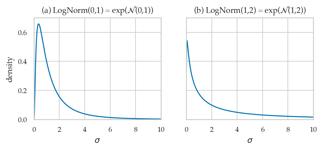

Choosing priors for the degrees of freedom parameter¶

# FIGURES ONLY
from scipy.stats import gamma as gammadist
from scipy.stats import expon
from ministats import plot_pdf

with plt.rc_context({"figure.figsize":(6,2.2)}):
    fig, (ax1, ax2) = plt.subplots(1,2, sharey=True)

    # PLOT 1
    alpha, beta = 2, 0.1
    rv_nu = gammadist(a=2, scale=1/beta)
    plot_pdf(rv_nu, rv_name="ν", ax=ax1)
    ax1.set_title(f'(a) Gamma($\\alpha=${alpha}, $\\beta=${beta})')
    ax1.set_xlim(0, 100)

    # PLOT 2
    scale = 30
    rv_nu_exp = expon(scale=scale)
    plot_pdf(rv_nu_exp, rv_name="ν", ax=ax2)
    ax2.set_title(f'(b) Expon($\\lambda=$1/{scale})')
    ax2.set_xlim(0, 100)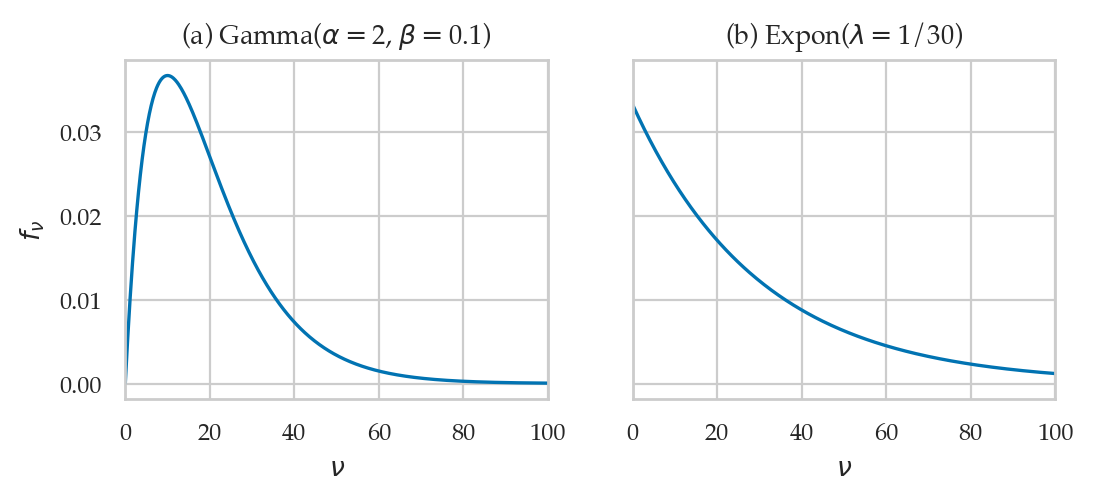

Example 1: comparing electricity prices¶

Electricity prices from East End and West End

Electricity prices dataset¶

eprices = pd.read_csv("datasets/eprices.csv")
eprices.groupby("loc")["price"].describe()

eprices["price"].mean(), eprices["price"].std()

(7.655555555555556, 1.973120020267162)

Bayesian model¶

\begin{align*} X_W \sim \mathcal{T}(\nu, M_W, \Sigma_W), \qquad \qquad X_E \sim \mathcal{T}(\nu, M_E, \Sigma_E), \qquad\qquad \\ M_W, M_E \!\sim\! \mathcal{N}(\mu_{M}, \sigma_{M}), \quad \log\Sigma_W, \log\Sigma_E\!\sim\!\mathcal{N}(0,1), \quad \nu \!\sim\! \text{Gamma}(2,0.1). \end{align*}

(3)

Bambi model¶

formula1 = bmb.Formula("price ~ 0 + loc",
                       "sigma ~ 0 + loc")

links1 = {"mu":"identity",
          "sigma":"log"}

priors1 = {
    "loc": bmb.Prior("Normal", mu=8, sigma=5),
    "sigma": {
        "loc": bmb.Prior("Normal", mu=0, sigma=1)
    },
    "nu": bmb.Prior("Gamma", alpha=2, beta=0.1),
}

mod1 = bmb.Model(formula=formula1,
                 family="t",
                 link=links1,
                 priors=priors1,
                 data=eprices)
mod1

       Formula: price ~ 0 + loc
                sigma ~ 0 + loc
        Family: t
          Link: mu = identity
                sigma = log
  Observations: 18
        Priors: 
    target = mu
        Common-level effects
            loc ~ Normal(mu: 8.0, sigma: 5.0)
        
        Auxiliary parameters
            nu ~ Gamma(alpha: 2.0, beta: 0.1)
    target = sigma
        Common-level effects
            sigma_loc ~ Normal(mu: 0.0, sigma: 1.0)

mod1.build()
mod1.graph()

Prior predictive checks¶

# TODO

Model fitting and analysis¶

idata1 = mod1.fit(random_seed=42)

Initializing NUTS using jitter+adapt_diag...
Multiprocess sampling (4 chains in 4 jobs)
NUTS: [nu, loc, sigma_loc]

Sampling 4 chains for 1_000 tune and 1_000 draw iterations (4_000 + 4_000 draws total) took 1 seconds.

Processing the results¶

Calculate derived quantities used for the analysis plots and summaries.

post1 = idata1["posterior"]

# Calculate sigmas from log-sigmas
#######################################################
logsig_W = post1["sigma_loc"].sel(sigma_loc_dim="West")
logsig_E = post1["sigma_loc"].sel(sigma_loc_dim="East")
post1["sigma_West"] = np.exp(logsig_W)
post1["sigma_East"] = np.exp(logsig_E)

# Calculate the difference between between means
post1["mu_West"] = post1["loc"].sel(loc_dim="West")
post1["mu_East"] = post1["loc"].sel(loc_dim="East")
post1["dmeans"] = post1["mu_West"] - post1["mu_East"]

# Calculate the difference between standard deviations
post1["dsigmas"] = post1["sigma_West"]-post1["sigma_East"]

# Effect size
#######################################################
pvar =(post1["sigma_West"]**2+post1["sigma_East"]**2)/2
post1["cohend"] = post1["dmeans"] / np.sqrt(pvar)

# #ALT: use helper function
# from ministats import calc_dmeans_stats
# calc_dmeans_stats(idata1, group_name="loc")

az.summary(idata1, kind="stats", hdi_prob=0.90,
           var_names=["mu_West", "mu_East", "dmeans", "sigma_West", "sigma_East", "dsigmas", "nu", "cohend"])

from ministats import plot_dmeans_stats
plot_dmeans_stats(mod1, idata1, group_name="loc");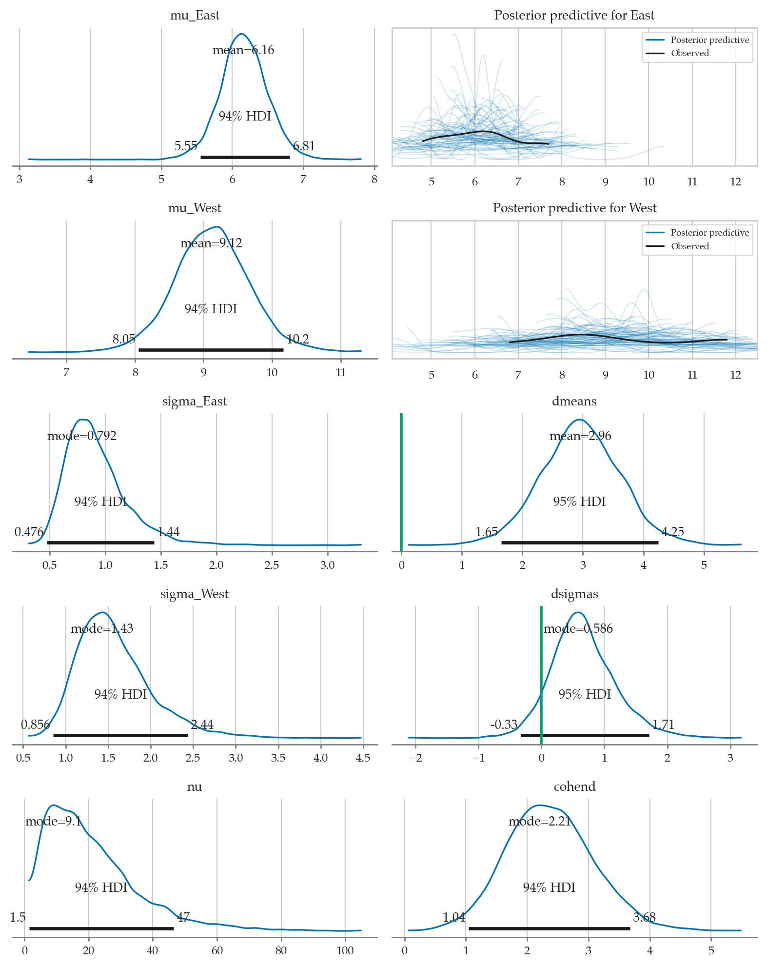

Compare to frequentist results¶

from scipy.stats import ttest_ind
pricesW = eprices[eprices["loc"]=="West"]["price"]
pricesE = eprices[eprices["loc"]=="East"]["price"]

res1 = ttest_ind(pricesW, pricesE, equal_var=False)
res1.statistic, res1.pvalue

(5.022875513276464, 0.00025703383372176116)

res1.confidence_interval(confidence_level=0.9)

ConfidenceInterval(low=1.9396575883681466, high=4.060342411631854)

from ministats import cohend2
cohend2(pricesW, pricesE)

2.3678062243290996

Conclusions¶

Example 2: comparing IQ scores¶

We’ll look at IQ scores data taken from a the paper Bayesian Estimation Supersedes the t-Test (BEST) by John K. Kruschke.

smart drug administered to treatment group and want to compare to control group. Data contains outliers)

cf. compare_iqs2_many_ways.ipynb

IQ scores dataset¶

iqs2 = pd.read_csv("datasets/iqs2.csv")
iqs2.groupby("group")["iq"].describe()

sns.stripplot(data=iqs2, x="iq", y="group", hue="group");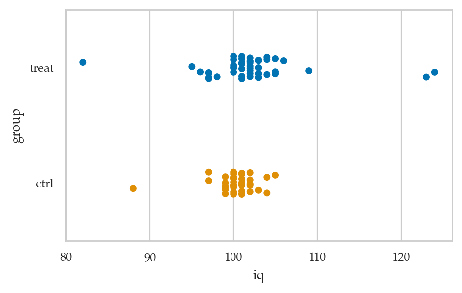

Bayesian model¶

TODO: add formulas

Bambi model¶

formula2 = bmb.Formula("iq ~ 0 + group",
                       "sigma ~ 0 + group")

priors2 = {
    "group": bmb.Prior("Normal", mu=100, sigma=35),
    "sigma": {
        "group": bmb.Prior("Normal", mu=1, sigma=2)
    },
    "nu": bmb.Prior("Gamma", alpha=2, beta=0.1),
}

mod2 = bmb.Model(formula=formula2,
                 family="t",
                 # link={"mu":"identity", "sigma":"log"}, # Bambi defaults
                 priors=priors2,
                 data=iqs2)

mod2

       Formula: iq ~ 0 + group
                sigma ~ 0 + group
        Family: t
          Link: mu = identity
                sigma = log
  Observations: 89
        Priors: 
    target = mu
        Common-level effects
            group ~ Normal(mu: 100.0, sigma: 35.0)
        
        Auxiliary parameters
            nu ~ Gamma(alpha: 2.0, beta: 0.1)
    target = sigma
        Common-level effects
            sigma_group ~ Normal(mu: 1.0, sigma: 2.0)

mod2.build()
mod2.graph()

Model fitting and analysis¶

idata2 = mod2.fit(random_seed=42)

Initializing NUTS using jitter+adapt_diag...
Multiprocess sampling (4 chains in 4 jobs)
NUTS: [nu, group, sigma_group]

Sampling 4 chains for 1_000 tune and 1_000 draw iterations (4_000 + 4_000 draws total) took 1 seconds.

from ministats import calc_dmeans_stats
calc_dmeans_stats(idata2, group_name="group");
az.summary(idata2, kind="stats", hdi_prob=0.95,
           var_names=["mu_treat", "mu_ctrl", "dmeans", "sigma_treat", "sigma_ctrl", "dsigmas", "nu", "cohend"])

from ministats import plot_dmeans_stats
plot_dmeans_stats(mod2, idata2, group_name="group", ppc_xlims=[82,124]);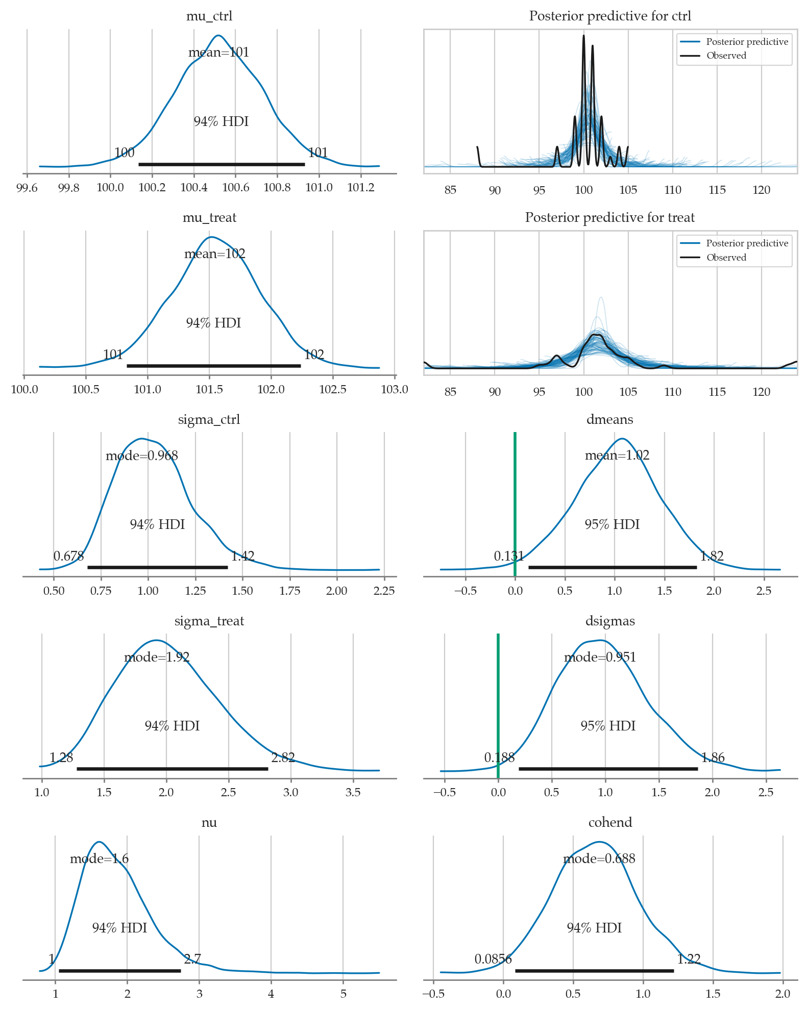

Sensitivity analysis¶

from ministats.book.tables import sens_analysis_dmeans_iqs2
results = sens_analysis_dmeans_iqs2(iqs2)
results

Compare to frequentist results¶

from scipy.stats import ttest_ind

treated = iqs2[iqs2["group"]=="treat"]["iq"]
controls = iqs2[iqs2["group"]=="ctrl"]["iq"]

res2 = ttest_ind(treated, controls, equal_var=False)
res2.statistic, res2.pvalue

(1.622190457290228, 0.10975381983712836)

res2.confidence_interval(confidence_level=0.95)

ConfidenceInterval(low=-0.36118477236636837, high=3.4766862921232016)

from ministats import cohend2
cohend2(treated, controls)

0.33096545301397307

# MAYBE
# # Test if the variances of the two groups are the same
# from scipy.stats import levene
# levene(treated, controls)

Conclusions¶

Explanations¶

Alternative choices of priors¶

e.g. prior for sigma as very wiiiiiide, and nu ~ Exp(1/29)+1 → BEST Bayesian estimation supersedes the t-test by John K. Kruschke

If we use a model with common standard deviation, we get equivalent of pooled sigma

# TODO

Performance tests¶

Simulated datasets¶

Simulate datasets with various combinations of $n$ , $\Delta$ , and outliers.

from ministats.book.tables import gen_dmeans_datasets

ns = [20, 30, 50, 100]
Deltas = [0, 0.2, 0.5, 0.8, 1.3]
outliers_options = ["no", "few", "lots"]
dataset_specs = gen_dmeans_datasets(ns=ns,
                                    Deltas=Deltas,
                                    outliers_options=outliers_options)
dataset_specs[0:4]

[{'n': 20, 'Delta': 0, 'outliers': 'no', 'random_seed': 45},
 {'n': 20, 'Delta': 0, 'outliers': 'few', 'random_seed': 46},
 {'n': 20, 'Delta': 0, 'outliers': 'lots', 'random_seed': 47},
 {'n': 20, 'Delta': 0.2, 'outliers': 'no', 'random_seed': 48}]

Model comparisons¶

Compare results several models:

Classical permutation test (from Section 4.5)
Classical Welch’s two-sample t-test (from Section 4.5)
Bayesian model with $\mathcal{N}$ data model
Robust Bayesian model with $\mathcal{T}$ data model
Bayes factors with JZS prior and standard cutoff

from ministats.book.tables import fit_dmeans_models
help(fit_dmeans_models)

Help on function fit_dmeans_models in module ministats.book.tables:

fit_dmeans_models(dataset, random_seed=42)
    Fit the following models for the difference of two means:
    - Permutation test from Section 3.5
    - Welch's two-sample $t$-test from Section 3.5
    - Bayesian model that uses normal as data model
    - Robust Bayesian model that uses t-distribution as data model
    - Bayes factor using JZS prior (using `pingouin` library)
    For each model, we run the hypothesis test to decide if the populations
    are the same or different based on the conventional cutoff level of 5%.
    We also construct a 90% interval estimates for the unknown `Delta`.

Results¶

# Download simdata/ directory if necessary
from ministats import ensure_simdata
ensure_simdata()

# Option A: load results from simulation
filename = "dmeans_perf_metrics__" \
            + "ns_20_30_50_100__" \
            + "Deltas_0_0.2_0.5_0.8_1.3__" \
            + "outs_no_few_lots__reps_100.csv"
results = pd.read_csv(os.path.join("simdata", filename), index_col=[0,1])
results.head(3)
# Option B: run full simulation (takes about three days)
# from ministats.book.tables import calc_dmeans_perf_metrics
# results = calc_dmeans_perf_metrics(reps=100)

simdata/ directory present and ready.

Type I (false positive) error rates¶

from ministats.book.tables import get_perf_table_typeI

tableA = get_perf_table_typeI(results)
tableA

Observations:

all models are about the same
BF model has significantly less false positives

Power analysis¶

from ministats.book.tables import get_perf_table_power

tableB = get_perf_table_power(results, show_all=False)
tableB

Observations:

Bayes $\mathcal{T}$ has higher power than Bayes $\mathcal{N}$
Bayes $\mathcal{T}$ outperforms all other models when outliers are present

Interval estimates coverage¶

from ministats.book.tables import get_perf_table_coverage

tableC = get_perf_table_coverage(results)
tableC

Observations:

All methods have coverage close to the nominal 90%
Bayes $\mathcal{T}$ produces narrower intervals

Discussion¶

Comparison to the frequentist two-sample t-test¶

results numerically similar
note we’re using 𝒯 as data model, not as a sampling distribution
conceptually different:
- p-value vs. decision based on posterior distribution
- confidence intervals vs. credible intervals

Comparing multiple groups¶

?Extension to Bayesian ANOVA? Can extend approach to multiple groups: Bayesian ANOVA

FWD reference to hierarchical models for group comparison covered in Section 5.5

Exercises¶

Exercise 1: small samples¶

As = [5.77, 5.33, 4.59, 4.33, 3.66, 4.48]
Bs = [3.88, 3.55, 3.29, 2.59, 2.33, 3.59]
groups = ["A"]*len(As) + ["B"]*len(Bs)
df1 = pd.DataFrame({"group": groups, "vals": As + Bs})
# df1

Exercise 2: lecture and debate curriculums¶

students = pd.read_csv("datasets/students.csv")
# students.groupby("curriculum")["score"].describe()

formula_std = bmb.Formula("score ~ 0 + curriculum",
                          "sigma ~ 0 + curriculum")
priors_std = {
    "curriculum": bmb.Prior("Normal", mu=70, sigma=30),
    "sigma": {
        "curriculum":bmb.Prior("Normal", mu=1, sigma=2)
    },
    "nu": bmb.Prior("Gamma", alpha=2, beta=0.1),
}
mod_std = bmb.Model(formula=formula_std,
                 family="t",
                 link="identity",
                 priors=priors_std,
                 data=students)
mod_std
# mod_std.build()
# mod_std.graph()

       Formula: score ~ 0 + curriculum
                sigma ~ 0 + curriculum
        Family: t
          Link: mu = identity
                sigma = log
  Observations: 15
        Priors: 
    target = mu
        Common-level effects
            curriculum ~ Normal(mu: 70.0, sigma: 30.0)
        
        Auxiliary parameters
            nu ~ Gamma(alpha: 2.0, beta: 0.1)
    target = sigma
        Common-level effects
            sigma_curriculum ~ Normal(mu: 1.0, sigma: 2.0)

idata_std = mod_std.fit(random_seed=42)

Initializing NUTS using jitter+adapt_diag...
Multiprocess sampling (4 chains in 4 jobs)
NUTS: [nu, curriculum, sigma_curriculum]

Sampling 4 chains for 1_000 tune and 1_000 draw iterations (4_000 + 4_000 draws total) took 1 seconds.

# Calculate the difference between between means
currs = idata_std["posterior"]["curriculum"]
mu_debate = currs.sel(curriculum_dim="debate")
mu_lecture = currs.sel(curriculum_dim="lecture")
idata_std["posterior"]["dmeans"] = mu_debate - mu_lecture
az.summary(idata_std, kind="stats", var_names=["dmeans"], hdi_prob=0.95)

# from ministats import plot_dmeans_stats
# plot_dmeans_stats(mod_std, idata_std, ppc_xlims=[50,100], group_name="curriculum");

# from scipy.stats import ttest_ind
# scoresD = students[students["curriculum"]=="debate"]["score"]
# scoresL = students[students["curriculum"]=="lecture"]["score"]
# res_std = ttest_ind(scoresD, scoresL, equal_var=False)
# res_std.statistic, res_std.pvalue
# from ministats import cohend2
# cohend2(scoresL, scoresD)

Exercise 3: redo exercises from Section 3.5 section using Bayesian methods¶

# TODO

Links¶

TODO

BONUS Examples¶

Example 4: small example form BEST vignette¶

See http://cran.nexr.com/web/packages/BEST/vignettes/BEST.pdf#page=2

# y1s = [5.77, 5.33, 4.59, 4.33, 3.66, 4.48]
# y2s = [3.88, 3.55, 3.29, 2.59, 2.33, 3.59]

# from ministats.bayes import bayes_dmeans
# mod4, idata4 = bayes_dmeans(y1s, y2s, groups=["y1", "y2"])

# from ministats import calc_dmeans_stats
# calc_dmeans_stats(idata4)
# az.summary(idata4, kind="stats", hdi_prob=0.95,
#            var_names=["dmeans", "sigma_y1", "sigma_y2", "dsigmas", "nu", "cohend"])

# from ministats import plot_dmeans_stats
# plot_dmeans_stats(mod4, idata4, ppc_xlims=None);

Example 5: comparing morning to evening¶

examples/paired_samples.py

# morning = [8.99, 9.21, 9.03, 9.15, 8.68, 8.82, 8.66, 8.82, 8.59, 8.14,
#            9.09, 8.80, 8.18, 9.23, 8.55, 9.03, 9.36, 9.06, 9.57, 8.38]
# evening = [9.82, 9.34, 9.73, 9.93, 9.33, 9.41, 9.48, 9.14, 8.62, 8.60,
#            9.60, 9.41, 8.43, 9.77, 8.96, 9.81, 9.75, 9.50, 9.90, 9.13]

# from ministats.bayes import bayes_dmeans
# mod5, idata5 = bayes_dmeans(evening, morning, groups=["evening", "morning"])

# from ministats import calc_dmeans_stats
# calc_dmeans_stats(idata5)
# az.summary(idata5, kind="stats", hdi_prob=0.95,
#            var_names=["dmeans", "sigma_evening", "sigma_morning", "dsigmas", "nu", "cohend"])

# from ministats import plot_dmeans_stats
# plot_dmeans_stats(mod5, idata5, ppc_xlims=None);