This notebook contains all the code examples from Section 2.5 Multiple continuous random variables of the No Bullshit Guide to Statistics.
Notebook setup
We’ll start by importing the Python modules we’ll need for this notebook.
# Ensure required Python modules are installed
%pip install --quiet numpy scipy seaborn ministats
[notice] A new release of pip is available: 26.0.1 -> 26.2
[notice] To update, run: pip install --upgrade pip
Note: you may need to restart the kernel to use updated packages.
# load Python modules
import numpy as np
import seaborn as sns
import matplotlib.pyplot as plt
# Figures setup
plt.clf() # needed otherwise `sns.set_theme` doesn't work
sns.set_theme(
context="paper",
style="whitegrid",
palette="colorblind",
rc={"font.family": "serif",
"font.serif": ["Palatino", "DejaVu Serif", "serif"],
"figure.figsize": (7,2)},
)
%config InlineBackend.figure_format = "retina"<Figure size 640x480 with 0 Axes># Simple float __repr__
import numpy as np
if int(np.__version__.split(".")[0]) >= 2:
np.set_printoptions(legacy='1.25')Joint probability density function
Example 1: bivariate normal distribution
TODO: formula for general bivarate normal
from scipy.stats import multivariate_normal

# Model parameters
muX, muY, sigmaX, sigmaY, rho = 10, 5, 3, 1, 0.75

# The mean vector
mu = [muX, muY]

# The covariance matrix
Sigma = [[         sigmaX**2,   rho*sigmaX*sigmaY ],
         [ rho*sigmaX*sigmaY,           sigmaY**2 ]]

# Computer model for the bivariate normal random variable
rvXY = multivariate_normal(mean=mu, cov=Sigma)rvXY.pdf((10,5))0.08020655225672235Probability of the event .
from scipy.integrate import dblquad

def fYX(y,x):
    """
    Adapter function because `dblquad` expects the function
    we're integrating to be of the form f(y,x), and not f(x,y).
    """
    return rvXY.pdf([x,y])


dblquad(fYX, a=10, b=14, gfun=5, hfun=7)[0]0.2905021692650627# ALT. using CDF
rvXY.cdf((14,7)) - rvXY.cdf((10,7)) - rvXY.cdf((14,5)) + rvXY.cdf((10,5))0.2905021692650628Unit total axiom
dblquad(fYX, a=-np.inf, b=np.inf, gfun=-np.inf, hfun=np.inf)[0]1.000000000045008TODO: formulas
from ministats import plot_joint_pdf_contourf

xlims = [3, 17]
ylims = [1.5, 8.5]

plot_joint_pdf_contourf(rvXY, xlims=xlims, ylims=ylims);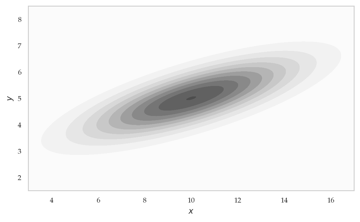
xlims = [3, 17]
ylims = [1.5, 8.5]
event = [(10,5), (14,7)]
ax = plot_joint_pdf_contourf(rvXY, xlims=xlims, ylims=ylims, highlight=[event]);
ax.text(12, 7.3, r"$\{10 \leq X \leq 14, 5 \leq Y \leq 7\}$", ha="center");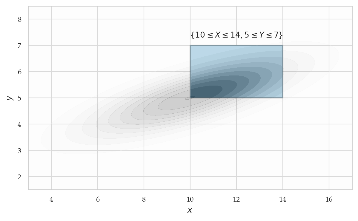
# ALT
from ministats import plot_joint_pdf_contour

xlims = [4, 16]
ylims = [3, 7]

plot_joint_pdf_contour(rvXY, xlims=xlims, ylims=ylims);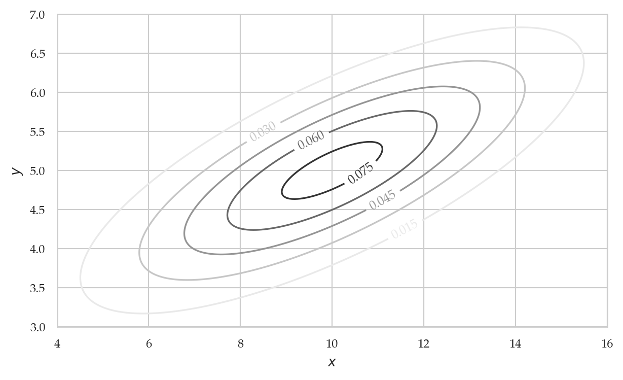
from ministats import plot_joint_pdf_surface

viewdict = dict(elev=60., azim=-110, roll=-16)
plot_joint_pdf_surface(rvXY, xlims=xlims, ylims=ylims, viewdict=viewdict);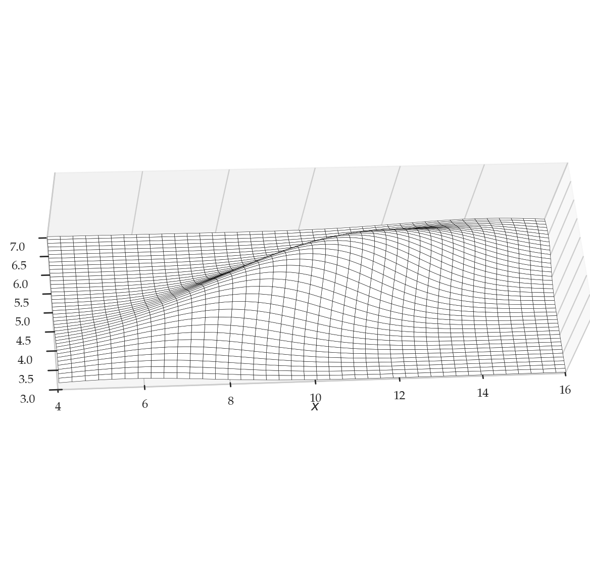
Marginal distribution functions
TODO: formulas
# Extract marginal f_X(x) = ∫ f_XY(x,y) dy
rvX = rvXY.marginal(dimensions=[0])
# rvX.pdf(1), rvX.cov[0][0]
xs = np.linspace(4, 16, 1000)
fXs = rvX.pdf(xs)
sns.lineplot(x=xs, y=fXs);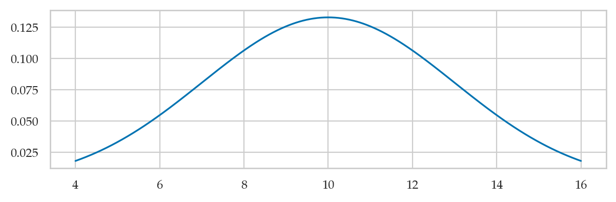
# ALT. compute marginal using integration
from scipy.integrate import quad

def fX(x):
    """
    Compute the marginal density  f_X(x) = ∫ f_XY(x,y) dy.
    """
    def fXY_at_x(y):
        return rvXY.pdf([x,y])
    return quad(fXY_at_x, a=-np.inf, b=np.inf)[0]

xs = np.linspace(4, 16, 500)
fXs = [fX(x) for x in xs]
sns.lineplot(x=xs, y=fXs);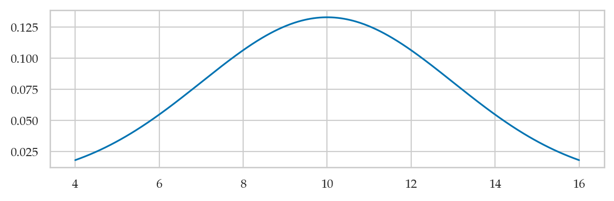
from ministats.book.figures import plot_joint_pdf_and_marginals

plot_joint_pdf_and_marginals(rvXY, xlims=xlims, ylims=ylims);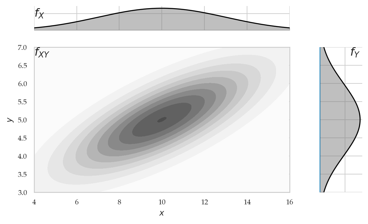
# Extract marginal f_Y(y) = ∫f_XY(x,y)dx
rvY = rvXY.marginal(dimensions=[1])
Conditional probability distributions
# ALT
from scipy.integrate import quad

def fYgivenX(y, x_a):
    """
    Compute the conditional distribtion f_Y|X(y|x=x_a).
    """
    rvX = rvXY.marginal(dimensions=[0])
    return rvXY.pdf([x_a,y]) / rvX.pdf(x_a)

ys = np.linspace(0, 10, 1000)

fYgivenX6s = [fYgivenX(y,x_a=6) for y in ys]
sns.lineplot(x=ys, y=fYgivenX6s, c="C0")

fYgivenX8s = [fYgivenX(y,x_a=8) for y in ys]
sns.lineplot(x=ys, y=fYgivenX8s, c="C1")

fYgivenX10s = [fYgivenX(y,x_a=10) for y in ys]
sns.lineplot(x=ys, y=fYgivenX10s, c="C2");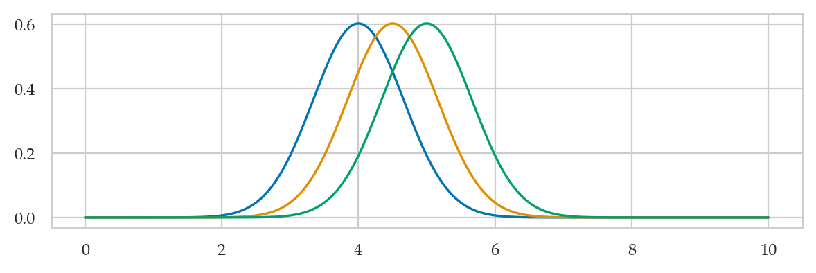
from ministats.book.figures import plot_slices_through_joint_pdf

xcuts = range(2, 15, 1)
plot_slices_through_joint_pdf(rvXY, xlims=[3,17], ylims=[0,10], xcuts=xcuts);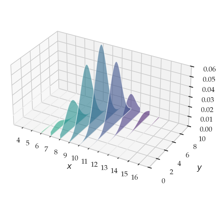
from ministats.book.figures import plot_conditional_fYgivenX

xcuts = range(6, 15, 1)
plot_conditional_fYgivenX(rvXY, xlims=[3,17], ylims=[0,10], xcuts=xcuts);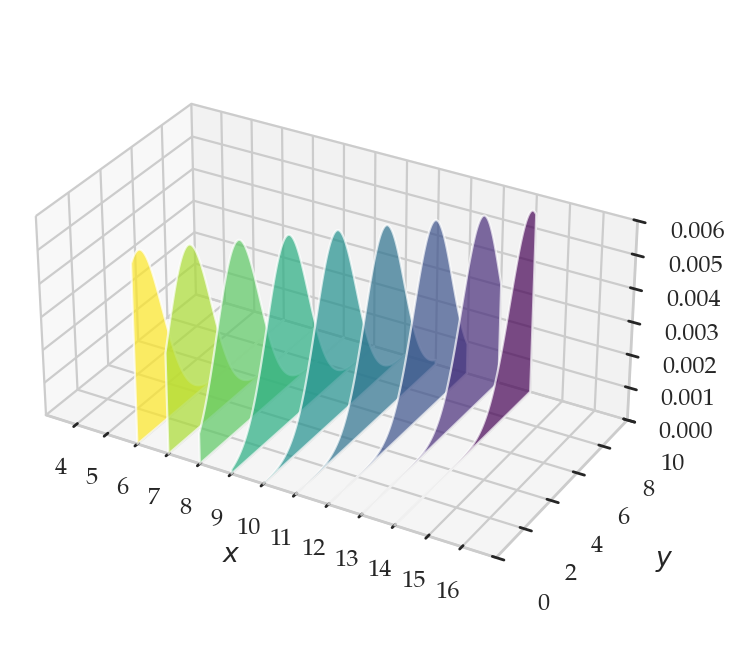
The chain rule
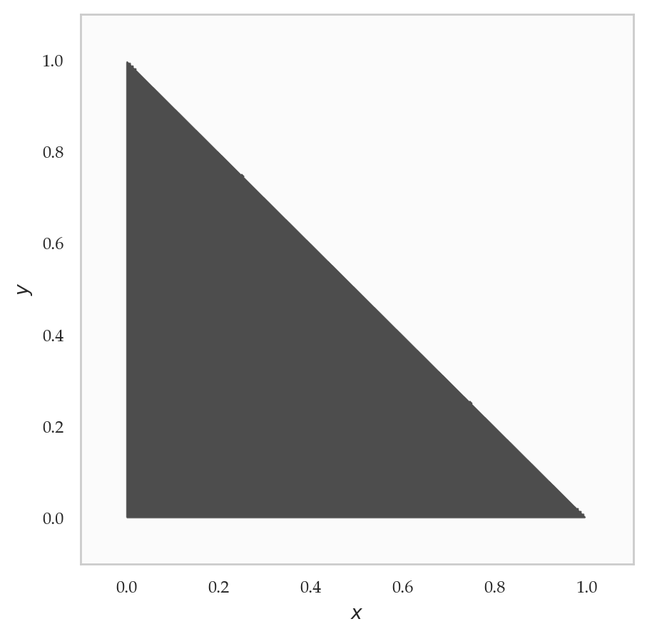
Example 2: bivariate uniform over a triangle
from ministats.probs import BivariateUniformOnTriangle

rvXY2 = BivariateUniformOnTriangle()
viewdict = dict(elev=60., azim=-110, roll=-16)
ax = plot_joint_pdf_surface(
rvXY2,
xlims=(-0.1, 1.1),
ylims=(-0.1, 1.1),
ngrid=2001,
viewdict=viewdict,
box_aspect=(1, 1, 0.5),
)
ax.set_zticks([0,1,2]);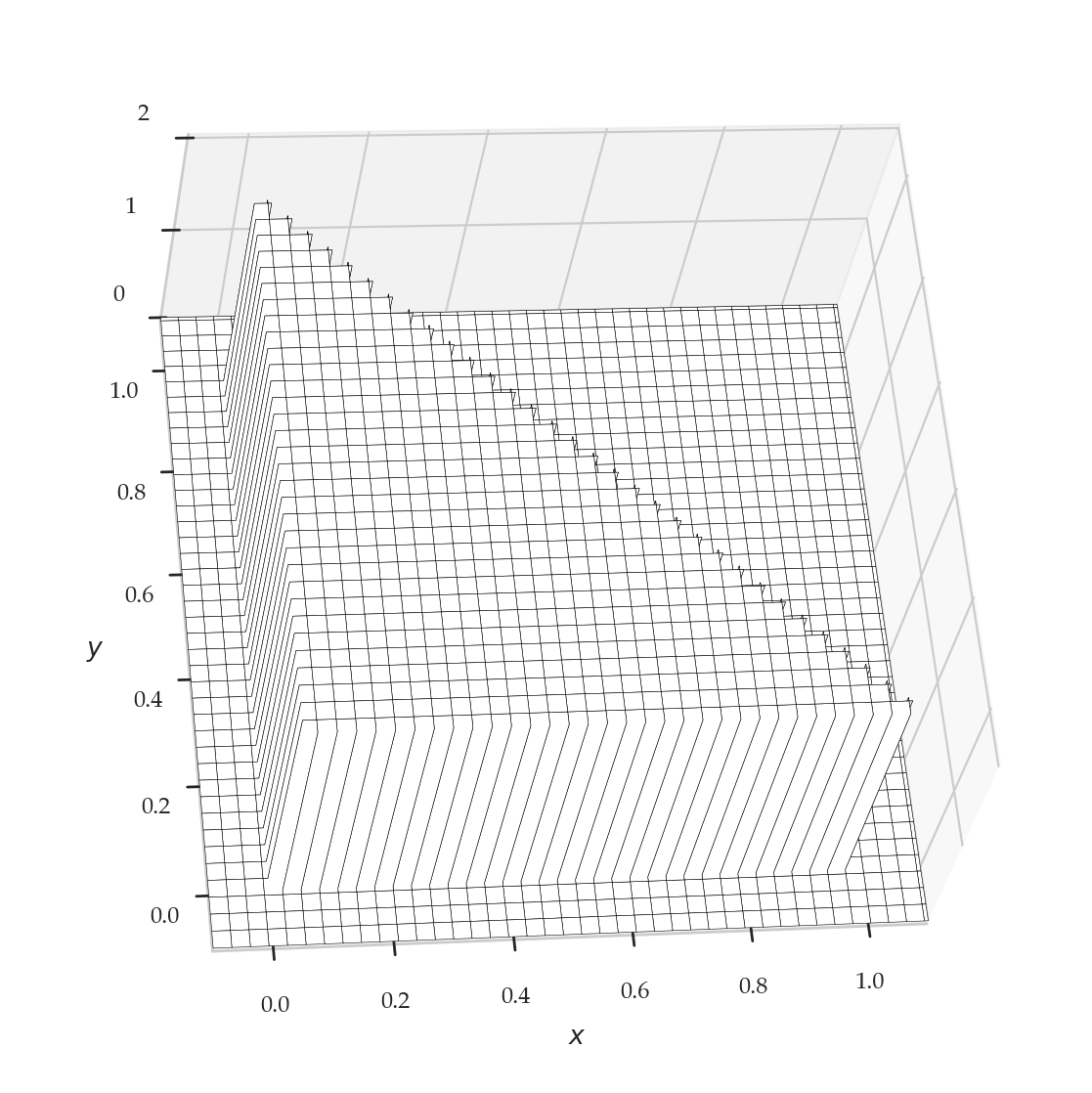
fig, ax = plt.subplots(figsize=(5, 5))
plot_joint_pdf_contourf(
    rvXY2,
    xlims=(-0.1, 1.1),
    ylims=(-0.1, 1.1),
    ngrid=401,
    ax=ax,
);
Checking Kolmogorov’s second axiom
from scipy.integrate import dblquad

def fYX2(y,x):
    """
    Adapter function because `dblquad` expects the function
    we're integrating to be of the form f(y,x), and not f(x,y).
    """
    return rvXY2.pdf([x,y])

def f1minusx(x):
    """
    A function that represents the upper boundary of the region
    of integration as a funciton of `x`.
    """
    return 1 - x

dblquad(fYX2, a=0, b=1, gfun=0, hfun=f1minusx)[0]1.0Computing probabilities
from scipy.integrate import dblquad

dblquad(fYX2, a=1/2, b=1, gfun=0, hfun=f1minusx)[0]0.25Marginal distributions
from ministats.book.figures import plot_joint_pdf_and_marginals

fig = plt.figure(figsize=(4,4))
plot_joint_pdf_and_marginals(
    rvXY2,
    xlims=(-0.1, 1.1),
    ylims=(-0.1, 1.1),
    ngrid=401,
    fig=fig);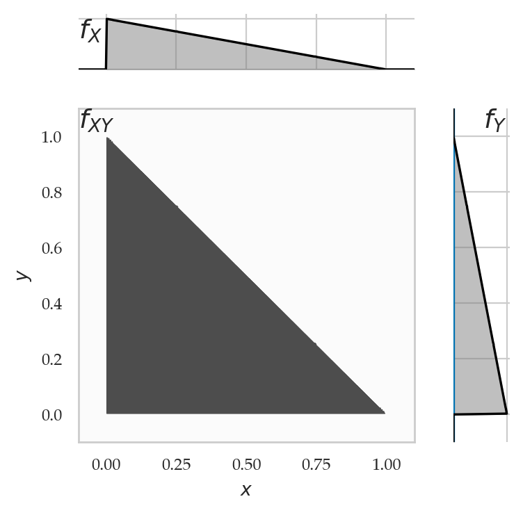
Conditional distributions
from ministats.book.figures import plot_joint_pdf_and_conditionals

plot_joint_pdf_and_conditionals(rvXY2, givenx=0.5, giveny=0.8);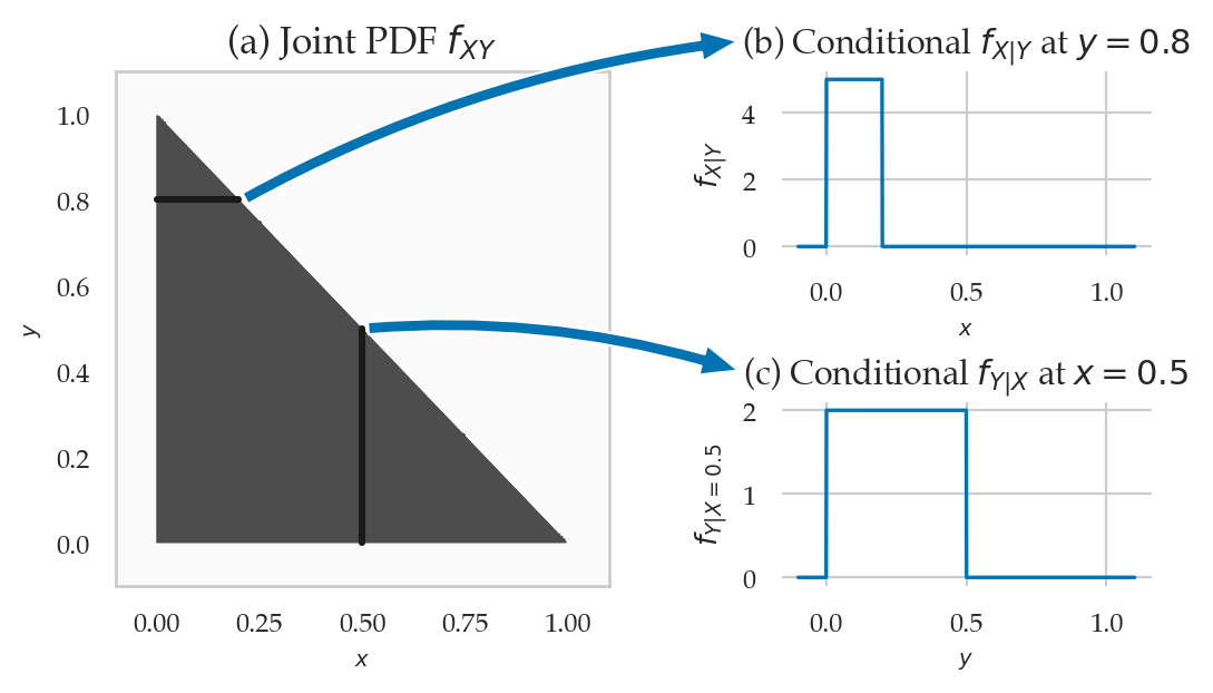
Bayes’ rule formula
Example 2 (continued): Bayes’ rule calculation
Multivariable expectation
Means
Covariance
Correlation
Example 1 revisited: computer model for the bivariate normal
Mean
rvXY.meanarray([10., 5.])Covariance
Sigma = rvXY.cov
Sigma
array([[9. , 2.25],
[2.25, 1. ]])covXY = Sigma[0,1]
covXY2.25Correlation
stdX = np.sqrt(Sigma[0,0])
stdY = np.sqrt(Sigma[1,1])

corrXY = covXY / (stdX * stdY)
corrXY0.75Independent random variables
TODO formulas