Analysis of variance (ANOVA) - No Bullshit Guide to Statistics

import matplotlib.pyplot as plt
import numpy as np
import seaborn as sns

%matplotlib inline
%config InlineBackend.figure_format = 'retina'

$\def\stderr#1{\mathbf{se}_{#1}}$ $\def\stderrhat#1{\hat{\mathbf{se}}_{#1}}$ $\def\Mean{\textbf{mean}}$ $\def\Var{\textbf{var}}$ $\def\Std{\textbf{std}}$ $\def\Freq{\textbf{freq}}$ $\def\RelFreq{\textbf{relfreq}}$ $\def\CI#1{\textbf{CI}_{#1}}$ $\def\CIL#1{\textbf{L}_{#1}}$ $\def\CIU#1{\textbf{U}_{#1}}$ $\def\ci#1{\textbf{ci}_{#1}}$ $\def\cil#1{\textbf{l}_{#1}}$ $\def\ciu#1{\textbf{u}_{#1}}$ $\def\DMeans{\textbf{dmeans}}$ $\def\Prop{\textbf{prop}}$ $\def\DProps{\textbf{dprops}}$ $\def\Err{ {\Large \varepsilon}}$ $\def\calN{\mathcal{N}}$ $\def\Tdist{\mathcal{T}}$ $\def\Expon{\mathrm{Expon}}$

(this cell contains the macro definitions like $\stderr{\overline{\mathbf{x}}}$ , $\stderrhat{}$ , $\Mean$ , ...)

Definitions¶

Formulas¶

Example¶

Explanations¶

Discussion¶

Equivalence between ANOVA and OLS¶

via https://stats.stackexchange.com/questions/175246/why-is-anova-equivalent-to-linear-regression

import numpy as np
from scipy.stats import randint, norm
np.random.seed(124)  # Fix the seed

x = randint(1,6).rvs(100) # Generate 100 random integer U[1,5]
y = x + norm().rvs(100)   # Generate my response sample

import pandas as pd
import seaborn as sns
df = pd.DataFrame({"x":x, "y":y})
sns.stripplot(data=df, x="x", y="y")
df.groupby("x")["y"].mean()

x
1    1.114427
2    1.958159
3    2.844082
4    4.198083
5    5.410594
Name: y, dtype: float64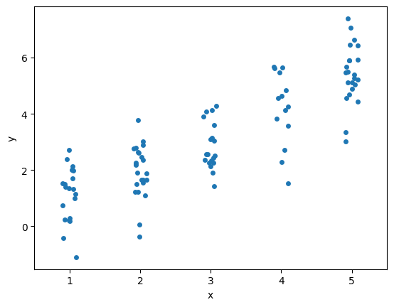

# One-way ANOVA
from scipy.stats import f_oneway

x1 = df[x==1]["y"]
x2 = df[x==2]["y"]
x3 = df[x==3]["y"]
x4 = df[x==4]["y"]
x5 = df[x==5]["y"]
res = f_oneway(x1, x2, x3, x4, x5)
res

F_onewayResult(statistic=62.07182379512491, pvalue=1.113218183344844e-25)

import statsmodels.api as sm
from statsmodels.formula.api import ols

# get ANOVA table as R like output
model = ols('y ~ C(x)', data=df).fit()
anova_table = sm.stats.anova_lm(model, typ=2)
anova_table

# MEANS
# 1    1.114427
# 2    1.958159
# 3    2.844082
# 4    4.198083
# 5    5.410594

# Ordinary Least Squares (OLS) model
model = ols('y ~ C(x)', data=df).fit()
model.summary()

betas = model.params.values
betas

array([1.11442735, 0.84373124, 1.72965468, 3.0836561 , 4.29616654])

scaled_batas = np.concatenate([[betas[0]], betas[0]+betas[1:]])
scaled_batas

array([1.11442735, 1.95815859, 2.84408203, 4.19808345, 5.41059388])

# Check if the two results are numerically equivalent
np.isclose(scaled_batas, df.groupby("x")["y"].mean().values)

array([ True, True, True, True, True])

# # Ordinary Least Squares (OLS) model (no intercept)
# model = ols('y ~ C(x) -1', data=df).fit()
# model.summary()

from scipy.stats.mstats import argstoarray
data = argstoarray(x1.values, x2.values, x3.values, x4.values, x5.values)

data.count(axis=1)
np.sum( data.count(axis=1) * ( data.mean(axis=1) - data.mean() )**2 )

250.9402371658938

# sswg manual compute
gmeans = data.mean(axis=1)
data_minus_gmeans = np.subtract(data.T, gmeans).T
(data_minus_gmeans**2).sum()

96.01507202947789

# sswg via parallel axis thm
gmeans = data.mean(axis=1)
np.sum( (data**2).sum(axis=1) - data.count(axis=1) * gmeans**2 )

96.01507202947788

from scipy.stats import f as fdist

def f_oneway(*args):
    """
    Performs a 1-way ANOVA, returning an F-value and probability given
    any number of groups.  From Heiman, pp.394-7.
    """
    # Construct a single array of arguments: each row is a group
    data = argstoarray(*args)
    ngroups = len(data)
    ntot = data.count()
    sstot = (data**2).sum() - (data.sum())**2/float(ntot)
    ssbg = (data.count(-1) * (data.mean(-1)-data.mean())**2).sum()
    sswg = sstot-ssbg
    print(ssbg, sswg, sstot)
    dfbg = ngroups-1
    dfwg = ntot - ngroups
    msb = ssbg/float(dfbg)
    msw = sswg/float(dfwg)
    f = msb/msw
    prob = fdist.sf(dfbg, dfwg, f)
    return f, prob

f_oneway(x1.values, x2.values, x3.values, x4.values, x5.values)

250.9402371658938 96.01507202947755 346.95530919537134

(62.07182379512513, 1.697371507321727e-08)