One-sample t-test for the mean

The goal of the one-sample $t$ -test to check if the mean $\mu$ of an unknown population $X \sim \mathcal{N}(\mu, \sigma_0)$ , equals the mean $\mu_0$ of a theoretical distribution $X_0 \sim \mathcal{N}(\mu_0, \sigma_0)$ . We’ll estimate the standard deviation $\sigma_0$ from the sample standard deviation $\mathbf{s}_{\mathbf{x}}$ . We discussed this hypothesis test in notebooks/34_analytical_approx.ipynb.

import matplotlib.pyplot as plt
import numpy as np
import seaborn as sns

%matplotlib inline
%config InlineBackend.figure_format = 'retina'

$\def\stderr#1{\mathbf{se}_{#1}}$ $\def\stderrhat#1{\hat{\mathbf{se}}_{#1}}$ $\def\Mean{\textbf{mean}}$ $\def\Var{\textbf{var}}$ $\def\Std{\textbf{std}}$ $\def\Freq{\textbf{freq}}$ $\def\RelFreq{\textbf{relfreq}}$ $\def\CI#1{\textbf{CI}_{#1}}$ $\def\CIL#1{\textbf{L}_{#1}}$ $\def\CIU#1{\textbf{U}_{#1}}$ $\def\ci#1{\textbf{ci}_{#1}}$ $\def\cil#1{\textbf{l}_{#1}}$ $\def\ciu#1{\textbf{u}_{#1}}$ $\def\DMeans{\textbf{dmeans}}$ $\def\Prop{\textbf{prop}}$ $\def\DProps{\textbf{dprops}}$ $\def\Err{ {\Large \varepsilon}}$ $\def\calN{\mathcal{N}}$ $\def\Tdist{\mathcal{T}}$ $\def\Expon{\mathrm{Expon}}$

(this cell contains the macro definitions like $\stderr{\overline{\mathbf{x}}}$ , $\stderrhat{}$ , $\Mean$ , ...)

Data¶

One sample of numerical observations $\mathbf{x}=[x_1, x_2, \ldots, x_n]$ .

Modeling assumptions¶

We model the unknown population as...

and the theoretical distribution is...

We assume the population is normally distributed $\textbf{(NORM)}$ , or the sample is large enough $\textbf{(LARGEn)}$ .

We also assume that the variance of the unknown population is known and equal to the variance of the theoretical population under $H_0$

Hypotheses¶

$H_0: \mu = \mu_0$ and $H_A: \mu \neq \mu_0$ , where $\mu$ is the unknown population mean, $\mu_0$ is the theoretical mean we are comparing to.

Statistical design¶

for $n=5$ ...

for $n=20$ ...

Estimates¶

Calculate the sample mean $\overline{\mathbf{x}} = \Mean(\mathbf{x})$ and the sample standard deviation $s_{\mathbf{x}} = \Std(\mathbf{x})$ . We can then calculate the estimated standard error of the mean $\stderrhat{\overline{\mathbf{x}}} = \frac{ s_{\mathbf{x}} }{ \sqrt{n} }$ .

Test statistic¶

Compute $t = \frac{\overline{\mathbf{x}} - \mu_0}{ \stderrhat{\overline{\mathbf{x}}} }$ from the sample mean $\overline{\mathbf{x}}$ , the theoretical population mean $\mu_0$ , the estimated standard error $\stderrhat{\overline{\mathbf{x}}}$ .

Sampling distribution¶

Student’s $t$ -distribution with $\nu=n-1$ degrees of freedom.

P-value calculation¶

from ministats import ttest_mean

%psource ttest_mean

def ttest_mean(sample, mu0, alt="two-sided"):
    """
    T-test to detect mean deviation from a population with known mean `mu0`.
    """
    assert alt in ["greater", "less", "two-sided"]
    obsmean = np.mean(sample)
    n = len(sample)
    std = np.std(sample, ddof=1)
    sehat = std / np.sqrt(n)
    obst = (obsmean - mu0) / sehat
    rvT = tdist(df=n-1)
    pvalue = tailprobs(rvT, obst, alt=alt)
    return pvalue

To perform the one-sample $t$ -test on the sample xs, we call ttest_mean(xs, mu0=...), with ... replaced by the expected mean $\mu_{X_0}$ of the theoretical population under $H_0$

Examples¶

For all the examples we present below, we assume the theoretical distribution we expect under the null hypothesis, is normally distributed with mean $\mu_{X_0}=100$ and standard deviation $\sigma_{X_0} = 5$ :

\texttt{rvX0} = X_0 \sim \mathcal{N}(100,5).

(1)

from scipy.stats import norm
muX0 = 100
sigmaX0 = 5
rvX0 = norm(muX0, sigmaX0)

Example A: population different from $H_0$ ¶

Suppose the unknown population is normally distributed with mean $\mu_{X_A}=104$ and standard deviation $\sigma_{X_A} = 3$ :

\texttt{rvXA} = X_A \sim \mathcal{N}(110,3).

(2)

muXA = 104
sigmaXA = 3
rvXA = norm(muXA, sigmaXA)

Let’s generate a sample xAs of size $n=20$ from the random variable $X = \texttt{rvXA}$ .

np.random.seed(42)

# generate a random sample of size n=20
n = 20
xAs = rvXA.rvs(n)
xAs

array([105.49014246, 103.5852071 , 105.94306561, 108.56908957,
       103.29753988, 103.29758913, 108.73763845, 106.30230419,
       102.59157684, 105.62768013, 102.60974692, 102.60281074,
       104.72588681,  98.26015927,  98.8252465 , 102.31313741,
       100.96150664, 104.942742  , 101.27592777,  99.7630889 ])

import seaborn as sns
with plt.rc_context({"figure.figsize":(7,1)}):
    sns.stripplot(x=xAs, jitter=0, alpha=0.5)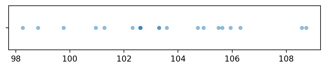

To obtain the $p$ -value, we first compute the observed $t$ -statistic, then calculate the tail probabilities in the two tails of the standard normal distribution $T_0 \sim \mathcal{T}(\nu)$ .

from scipy.stats import t as tdist

obsmean = np.mean(xAs)
std = np.std(xAs, ddof=1)
sehat = std / np.sqrt(n)
obst = (obsmean - muX0) / sehat
rvT0 = tdist(df=n-1)
pvalue = rvT0.cdf(-obst) + 1-rvT0.cdf(obst)
obst, pvalue

(5.413149619618617, 3.186228235607658e-05)

The helper function ttest_mean from the ministats module performs exactly the same sequence of steps to compute the $p$ -value.

from ministats import ttest_mean
ttest_mean(xAs, mu0=muX0)

3.1862282356088544e-05

The $p$ -value we obtain is 0.00003186, which is below the cutoff value $\alpha=0.05$ , so our conclusion is we reject the null hypothesis: the mean of the sample xAs is not statistically significantly different from the theoretically expected mean $\mu_{X_0} = 100$ .

Example B: sample from a population as expected under $H_0$ ¶

# unknown population X = X0
rvXB = norm(muX0, sigmaX0)

Let’s generate a sample xBs of size $n=20$ from the random variable $X = \texttt{rvX}$ , which has the same distribution as the theoretical distribution we expect under the null hypothesis.

# np.random.seed(32)  produces false positie
np.random.seed(31)

# generate a random sample of size n=20
n = 20
xBs = rvXB.rvs(n)
xBs

array([ 97.92621393,  98.33315666, 100.40545993,  96.04486524,
        98.90700164,  96.18401578,  96.11439878, 109.24678261,
        96.47199845,  99.56978983, 101.43966651,  99.34306739,
        95.08627924,  95.40604357, 105.99717245,  98.29312879,
        91.20696344, 100.25558735,  97.14035504,  96.49716979])

import seaborn as sns
with plt.rc_context({"figure.figsize":(7,1)}):
    sns.stripplot(x=xBs, jitter=0, alpha=0.5)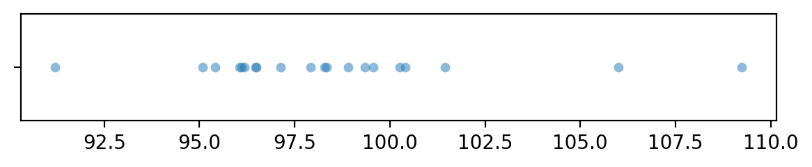

from ministats import ttest_mean
ttest_mean(xBs, mu0=muX0)

0.1013574486082352

The $p$ -value we obtain is 0.10, which is above the cutoff value $\alpha=0.05$ so our conclusion is that we’ve failed to reject the null hypothesis: the mean of the sample xBs is not significantly different from the theoretically expected mean $\mu_{X_0} = 100$ .

Confidence interval for the unknown mean¶

from ministats import ci_mean

The confidence interval for the unknown population mean $\mu_A$ in Example A is:

ci_mean(xAs, alpha=0.1, method='a')

[102.3725312980782, 104.59967733327082]

ci_mean(xBs, alpha=0.1, method='a')

[96.98044495642183, 100.00646668579604]

Effect size estimates¶

Use the one-sample $z$ -test if the population standard deviation is known

Data¶

Modeling assumptions¶

Hypotheses¶

Statistical design¶

Estimates¶

Test statistic¶

Sampling distribution¶

P-value calculation¶

Examples¶

Example A: population different from $H_0$ ¶

Example B: sample from a population as expected under $H_0$ ¶

Confidence interval for the unknown mean¶

Effect size estimates¶

Discussion¶

Links¶

Data¶

Modeling assumptions¶

Hypotheses¶

Statistical design¶

Estimates¶

Test statistic¶

Sampling distribution¶

P-value calculation¶

Examples¶

Example A: population different from H0H_0H0​¶

Example B: sample from a population as expected under H0H_0H0​¶

Confidence interval for the unknown mean¶

Effect size estimates¶

Related¶

Discussion¶

Links¶

Example A: population different from $H_0$ ¶

Example B: sample from a population as expected under $H_0$ ¶