Section 2.7 — Random variable generation

This notebook contains the code examples from Section 2.7 Random variable generation of the No Bullshit Guide to Statistics.

Notebook setup

# load Python modules
import numpy as np
import pandas as pd
import random
import seaborn as sns
import matplotlib.pyplot as plt

# Figures setup
sns.set_theme(
    context="paper",
    style="whitegrid",
    palette="colorblind",
    rc={'figure.figsize': (7,4)},
)

%config InlineBackend.figure_format = 'retina'

# set random seed for repeatability
random.seed(16)
np.random.seed(16)

Why simulate?

Running simulations of random variables is super useful:

• fake data generation

• probability calculations

• statistical procedures

(see book)

General procedure to simulate \(\mathbb{E}_X(g)\):

n = 30

gvalues = []
for i in range(0,n):
    xi = gen_x()
    gi = g(xi)
    gvalues.append(gi)

expg = sum(gvalues) / n

We’ll see different variations of this procedure (for loop that generates many random observations and does something with them).

Random variable generation using a computer

import random

random.random()

0.36152277491407514

# # ALT.
# import numpy as np
# np.random.rand()

Discrete random variable generation

Splitting up the uniform random variable …

Example 1: generating Bernoulli observations

Consider the Bernoulli random variable \(B \sim \textrm{Bernoulli}(p)\), which corresponds to a coin toss with probability of heads (outcome 1) equal to \(p\), and probability of tails (outcome 0) \((1-p)\).

The function gen_b defined below is a generator of observations from the random variable \(B\).

def gen_b(p=0.5):
    u = random.random()
    if u < p:
        return 1
    else:
        return 0

To generate a random observation from \(B \sim \textrm{Bernoulli}(p=0.3)\), we simply need to call the function gen_b with the keyword argument p=0.3.

gen_b(p=0.3)

0

Let’s now generates n=1000 observations from \(B \sim \textrm{Bernoulli}(p=0.3)\), and compute the proportion of the outcome \(1\) (heads) in the list.

n = 1000
bsample = [gen_b(p=0.3) for i in range(0,n)]
bsample.count(1) / n

0.316

# # ALT. Use regular for-loop, instead of list comprehension syntax
# n = 1000
# bsample = []
# for i in range(0,n):
#     b = gen_b(p=0.3)
#     bsample.append(b)
# bsample.count(1) / n

Continuous random variable generation

See the book or explanations of the the invers-CDF trick.

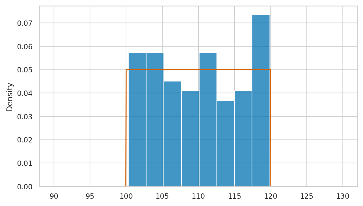
Example 2: generating observations from a shifted uniform distribution

\(V \sim \mathcal{U}(\alpha=100,\beta=120)\)

def gen_v():
    u = random.random()
    v = 100 + 20*u
    return v

gen_v()

107.26199234069637

n = 100
vsample = [gen_v() for i in range(0,n)]

vsample[0:3]  # first three observations

[103.6386436977451, 117.34140363667541, 113.35634072970831]

min(vsample), max(vsample)  # Range

(100.32987267319582, 119.88187770589093)

# plot a histogram of data in `vsample`
sns.histplot(vsample, stat="density")

# plot the pdf of the model
from scipy.stats import uniform
rvV = uniform(100,20)
xs = np.linspace(90,130,1000)
sns.lineplot(x=xs, y=rvV.pdf(xs), color="r")

<Axes: ylabel='Density'>

Example 3: generating observations from an exponential distribution

def gen_e(lam):
    u = random.random()
    e = -1 * np.log(1-u) / lam
    return e

Where lam is the \(\lambda\) (lambda) parameter chosen for exponential model family.

np.random.seed(6)

n = 1000  # number of observations to generate
esample = [gen_e(lam=0.2) for i in range(0,n)]

esample[0:3]  # first three observations

[0.5024273707608603, 10.625297726488984, 2.731193337322976]

# plot a histogram of data in `esample`
sns.histplot(esample, stat="density")

# plot the pdf of the model
from scipy.stats import expon
lam = 0.2
rvE = expon(0,1/lam)
xs = np.linspace(0,30,1000)
sns.lineplot(x=xs, y=rvE.pdf(xs), color="r")

<Axes: ylabel='Density'>

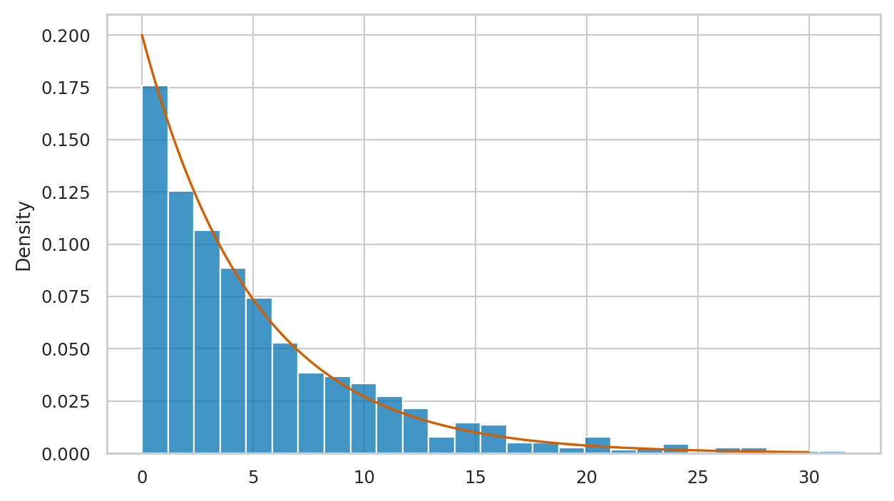
We’ll develop various way to analyze this “goodness of fit” between the sample esample data we generated and the theoretical model \(f_E\) in the remainder of this notebook.

Empirical distributions

Let’s write a function that compute the value empirical cumulative distribution (eCDF) of the sample data. The function takes two inputs: data the sample of observations, and b, the value where we want to evaluate the function.

def ecdf(data, b):
    sdata = np.sort(data)
    count = sum(sdata <= b)    # num. of obs. <= b
    return count / len(data)   # proportion of total

Note the sorting step is not strictly necessary, but it guarantees the sdata is a NymPy array object which allows the comparison to work.

ecdf(vsample, 110)

0.48

ecdf(esample, 5)

0.606

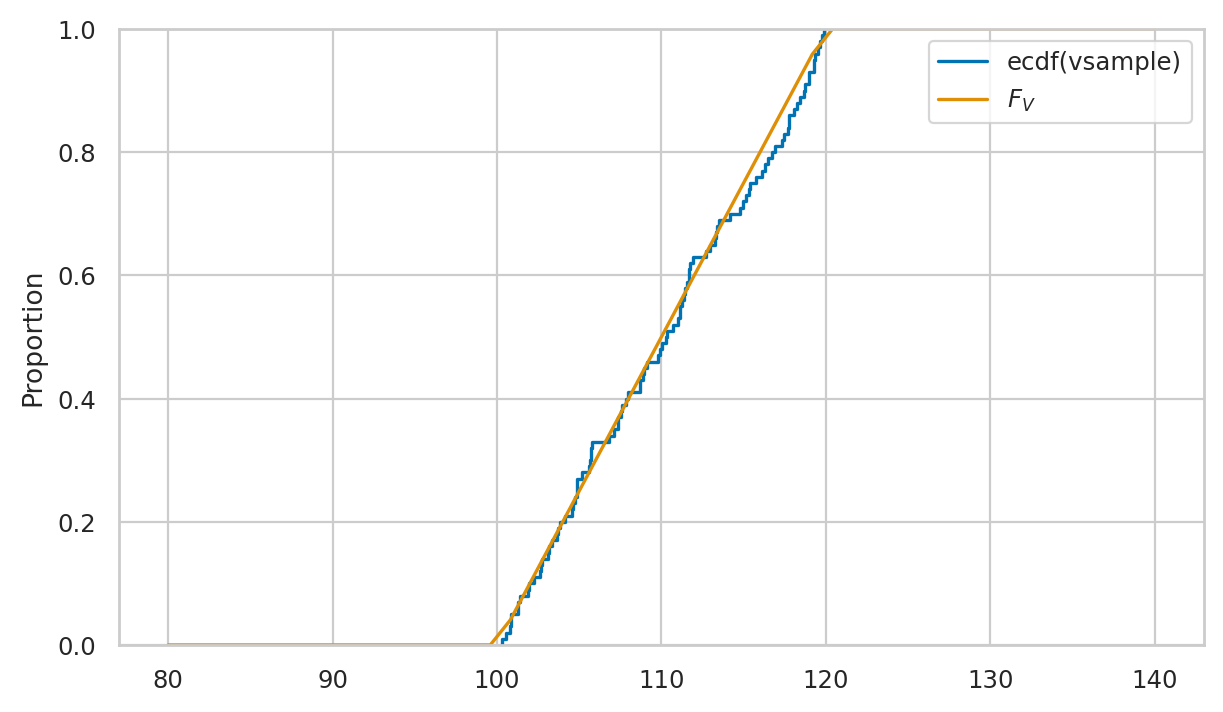
Visualizing the empirical cumulative distribution

sns.ecdfplot(vsample, label="ecdf(vsample)")

from scipy.stats import uniform
rvV = uniform(100,20)
bs = np.linspace(80,140)
sns.lineplot(x=bs, y=rvV.cdf(bs), label="$F_V$")

<Axes: ylabel='Proportion'>

# # ALT. manually plot ecdf using lineplot
# bs = np.linspace(80,140,1000)
# empFvs = [ecdf(vsample,b) for b in bs]
# sns.lineplot(x=bs, y=empFvs, drawstyle='steps-post')

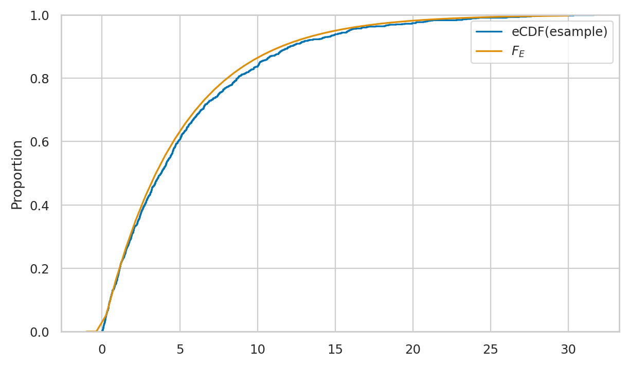
sns.ecdfplot(esample, label="eCDF(esample)")

bs = np.linspace(-1,30)
sns.lineplot(x=bs, y=rvE.cdf(bs), label="$F_E$")

<Axes: ylabel='Proportion'>

Measuring data-model fit

Want to measure if vsample comes from \(\mathcal{U}(100,120)\). Here are the first five values we simulated:

vsample[0:3]

[103.6386436977451, 117.34140363667541, 113.35634072970831]

We also want to check if the data we generated esample comes from \(\textrm{Expon}(\lambda=0.2)\).

esample[0:3]

[0.5024273707608603, 10.625297726488984, 2.731193337322976]

Let’s also generate an additional sample nsample from the normal distribution \(\mathcal{N}(1000,100)\) so we’ll be able to make a variety of comparisons.

np.random.seed(6)

from scipy.stats import norm
rvN = norm(1000, 100)
nsample = rvN.rvs(100)
nsample[0:3]

array([ 968.82163265, 1072.90039236, 1021.78207881])

Visual comparison between data and model distributions

Shifted uniform distribution

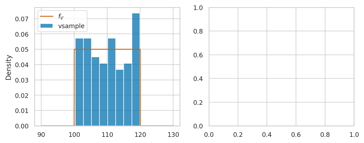
Here is the code for comparison of vsample and the theoretical model rvV \(= \mathcal{U}(100,120)\).

from scipy.stats import uniform
rvV = uniform(100,20)

fig, axs = plt.subplots(1,2, figsize=(8,3))
xs = np.linspace(90,130,1000)

# plot histogram of `vsample`
sns.histplot(vsample, stat="density", ax=axs[0], label="vsample")

# plot the pdf of rvV 
sns.lineplot(x=xs, y=rvV.pdf(xs), color="r", ax=axs[0], label="$f_V$")
lines, labels = axs[0].get_legend_handles_labels()
axs[0].legend(reversed(lines[0:2]), reversed(labels[0:2]))

# plot a empirical cumulative distribution
sns.ecdfplot(vsample, ax=axs[1], label="eCDF(vsample)")

# plot the CDF of rvV
sns.lineplot(x=xs, y=rvV.cdf(xs), color="r", ax=axs[1], label="$F_V$")
axs[1].set_ylim(-0.05, 1.05)

(-0.05, 1.05)

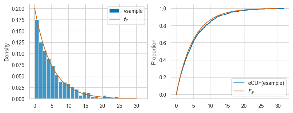
Exponential distribution

from scipy.stats import expon
lam = 0.2
rvE = expon(0,1/lam)

Here is the code for visual comparison of esample and the theoretical model rvE \(=\mathrm{Expon}(\lambda=0.2)\), based on the probability density and cumulative probability distributions.

fig, axs = plt.subplots(1,2, figsize=(8,3))
xs = np.linspace(0,30,1000)

# plot histogram of `esample`
sns.histplot(esample, stat="density", ax=axs[0], label="vsample")

# plot the pdf of rvE
sns.lineplot(x=xs, y=rvE.pdf(xs), color="r", ax=axs[0], label="$f_E$")
lines, labels = axs[0].get_legend_handles_labels()
axs[0].legend(reversed(lines[0:2]), reversed(labels[0:2]))

# plot a empirical cumulative distribution
sns.ecdfplot(esample, ax=axs[1], label="eCDF(esample)")

# plot the CDF of rvE
sns.lineplot(x=xs, y=rvE.cdf(xs), color="r", ax=axs[1], label="$F_E$")
axs[1].set_ylim(-0.05, 1.05)

(-0.05, 1.05)

Using Q-Q plots to compare quantiles

The quantile-quantile plot qqplot(data, dist) is used to compare the positions of the quantiles of the dataset data against the quantiles of the theoretical distribution dist, which is an instance of one of the probability models in scipy.stats.

The easiest way to generate a Q-Q plot is to use the function qqplot defined in the the statsmodels package.

from statsmodels.graphics.api import qqplot

Examples of good fit

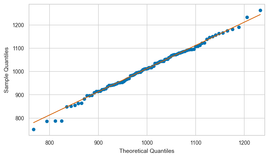
Normal data vs. the true normal model

Let’s look at the quantiles of the data in nsample, plotted versus the quantiles of the theoretical model \(\mathcal{N}(1000,100)\).

qqplot(nsample, dist=norm(1000,100), line='q');

Normal data vs. the standard normal

qqplot(nsample, dist=norm(0,1), line='q');

Examples of bad fit

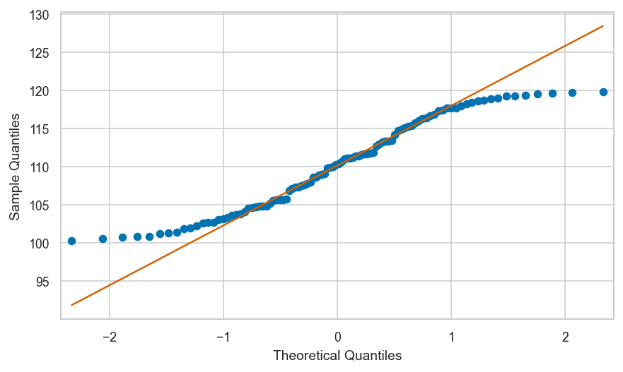
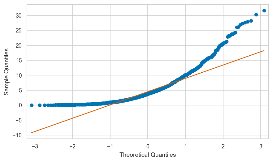
Shifted uniform data vs. standard normal

vsample = np.array(vsample)
qqplot(vsample, dist=norm(0,1), line="q");

Exponential data vs. standard normal

esample = np.array(esample)
qqplot(esample, dist=norm(0,1), line="q");

Note the lowest quantiles don’t match (exponential data limited to zero), and the high quantiles don’t match either (exponential data has a long tail).

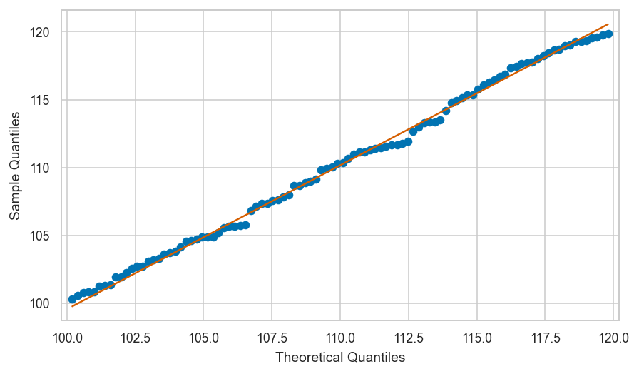
Shifted uniform sample vs. true model

vsample = np.array(vsample)
qqplot(vsample, dist=rvV, line="q");

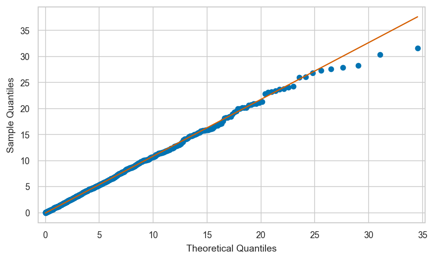
Exponential sample vs. true exponential model

qqplot(esample, dist=rvE, line="q");

Generating a Q-Q plot manually (bonus material)

If want to know how the Q-Q plot is generated, you can look at the following function qq_plot which the same way as qqplot.

def qq_plot(sample, dist, line="q"):
    qs = np.linspace(0, 1, len(sample))
    xs = dist.ppf(qs)
    ys = np.quantile(sample, qs)
    ax = sns.scatterplot(x=xs, y=ys, alpha=0.2)
    if line == "q":
        # compute the parameters m and b for the diagonal
        xq25, xq75 = dist.ppf([0.25, 0.75])
        yq25, yq75 = np.quantile(sample, [0.25,0.75])
        m = (yq75-yq25)/(xq75-xq25)
        b = yq25 - m * xq25
        # add the line  y = m*x+b  to the plot
        linexs = np.linspace(min(xs[1:]),max(xs[:-1]))
        lineys = m*linexs + b
        sns.lineplot(x=linexs, y=lineys, ax=ax, color="r")
    return ax

# # ALT2. use the `probplot` from the `scipy.stats` module
# from scipy.stats import probplot
# probplot(nsample, dist=norm(1000,100), plot=plt)

Comparing moments

A simple way to measure how well the data sample \(\mathbf{x} = (x_1, x_2, \ldots , x_n)\) fits the probability model \(f_X\) is to check if the data distribution and the probability distribution have the same moments.

In order to easily be able to calculate the moments of the data samples, we’ll convert vsample and esample into Pandas series objects, which have all the necessary methods.

vseries = pd.Series(vsample)
eseries = pd.Series(esample)

Moments of uniform distribution

vseries.mean(), rvV.mean()

(110.21271847666772, 110.0)

vseries.var(), rvV.var()

(35.95736108409104, 33.33333333333333)

Let’s now compare the skew of dataset and the skew of the distribution:

vseries.skew(), rvV.stats("s")

(0.03970716302600479, 0.0)

Finally, let’s compare the kurtosis of dataset and the kurtosis of the distribution.

vseries.kurt(), rvV.stats("k")

(-1.2584390506748377, -1.2)

Moments of exponential distribution

eseries.mean(), rvE.mean()

(5.343224374466268, 5.0)

eseries.var(), rvE.var()

(27.53085874882216, 25.0)

Let’s now compare the skew of dataset and the skew of the distribution:

eseries.skew(), rvE.stats("s")

(1.7338627932228903, 2.0)

Finally, let’s compare the kurtosis of dataset and the kurtosis of the distribution.

eseries.kurt(), rvE.stats("k")

(3.557504048617028, 6.0)

Example of bad fit between higher moments

Define the random variable rvNE as the best normal approximation to random variable rvE.

rvNE = norm(5,5)
rvNE.mean(), rvNE.var()

(5.0, 25.0)

eseries.skew(), rvNE.stats("s")

(1.7338627932228903, 0.0)

eseries.kurt(), rvNE.stats("k")

(3.557504048617028, 0.0)

Kolmogorov–Smirnov test

from scipy.stats import ks_1samp

Let’s jump right ahead and compute the KS distance for the data and distribution of interest.

ks_1samp(nsample, rvN.cdf).statistic

0.07815466189999987

ks_1samp(esample, rvE.cdf).statistic

0.03597247001342496

ks_1samp(vsample, rvV.cdf).statistic

0.05707018183377044

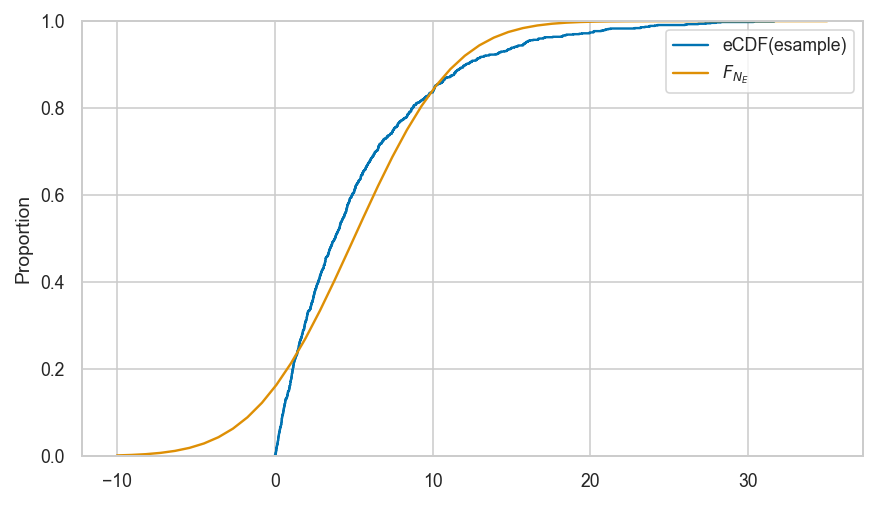
Example of big distance

ks_1samp(esample, rvNE.cdf).statistic

0.15871546070321535

sns.ecdfplot(esample, label="eCDF(esample)")
bs = np.linspace(-10,35)
sns.lineplot(x=bs, y=rvNE.cdf(bs), label="$F_{N_E}$")

<Axes: ylabel='Proportion'>

KS distances after standardization (optional)

Define the function standardize that transforms any dataset so it will have mean zero, and standard deviation one.

def standardize(data):
    xbar = data.mean()
    s = data.std()
    return (data-xbar)/s

# ALT. Use existing function that does the same as `standardize`
from scipy.stats import zscore

We can now report the KS distances, between the standardized version so nsample, esample, and vsample and standard normal \(\mathcal{N}(0,1)\), to check how “normal” they are.

ks_1samp(zscore(nsample), norm(0,1).cdf).statistic

0.037541386171241364

ks_1samp(zscore(vsample), norm(0,1).cdf).statistic

0.10026891576437313

ks_1samp(zscore(esample), norm(0,1).cdf).statistic

0.15419311135216357

data = expon(0,10).rvs(100)
ks_1samp(zscore(data), norm(0,1).cdf).statistic

0.1781210103950946

Calculating the KS distance manually (optional)

The computation is a little tricky since the eCDF is a stepwise function, so we need to two differences \(|F_X(x_i) - F_{\mathbf{x}}(x_i)|\) and \(|F_X(x_i) - F_{\mathbf{x}}(x_{i-1})|\).

def ks_dist(sample, rv=norm(0,1)):
    """
    Compute the KS distance between observed data in `sample`
    and the theoretical distribution of random variable `rv`.
    """
    sample = sorted(sample)
    ks_dists = []

    x0 = sample[0]
    ks_dist0 = rv.cdf(x0)
    ks_dists.append(ks_dist0)

    n = len(sample)
    for i in range(1,n):
        # xi
        xi = sample[i]
        eCDFxi = ecdf(sample, b=xi)
        ks_dist1 = abs(eCDFxi - rv.cdf(xi))
        ks_dists.append(ks_dist1)
        # x(i-1)
        xim1 = sample[i-1]
        eCDFxim1 = ecdf(sample, b=xim1)
        ks_dist2 = abs(eCDFxim1 - rv.cdf(xi))
        ks_dists.append(ks_dist2)

    # find max
    max_ks_dist = max(ks_dists)
    return max_ks_dist

Test 1

ks_dist(nsample, rv=norm(1000,100))

0.07815466189999987

ks_1samp(nsample, norm(1000,100).cdf).statistic

0.07815466189999987

Test 2

ks_dist(standardize(nsample), rv=norm(0,1))

0.037541386171241364

ks_1samp(standardize(nsample), norm(0,1).cdf).statistic

0.037541386171241364

Bootstrap sample generation

from scipy.stats import norm
rvN = norm(1000, 100)

np.random.seed(72)
sample = rvN.rvs(30)
sample

array([1031.85454991,  932.04405655,  779.16115305, 1059.02401628,
       1167.47660438,  833.40440269,  917.56612626, 1054.52603422,
       1000.11861932,  924.29694777, 1062.95451919,  990.43682345,
        849.21393503,  949.99869847, 1171.40102725,  877.62327349,
       1139.59050836, 1041.44763431, 1151.96667669, 1139.0063404 ,
        891.5999061 ,  957.46318231,  937.81775307, 1145.86005158,
        872.50054515, 1112.86094852, 1179.05765281,  948.13164741,
        932.89197563, 1073.67607886])

print([round(val, 2) for val in sample[0:4]])

[1031.85, 932.04, 779.16, 1059.02]

sample.mean()

1004.1657229506349

Let’s generate a bootstrap sample and compute its mean:

bsample = np.random.choice(sample,30)
bsample.mean()

989.8642131674898

Let’s compute the means of \(10\) bootstrap samples:

B = 10
bmeans = []
for k in range(0,B):
    bsample = np.random.choice(sample, 30)
    bmean = bsample.mean() 
    bmeans.append(bmean)

# bmeans

print([round(bmean, 2) for bmean in bmeans])

[1002.72, 968.09, 995.78, 964.45, 1011.08, 1013.17, 1027.03, 1041.01, 969.77, 1029.55]

max(abs(bmeans - sample.mean()))

39.719674810092215

# # BONUS: draw B=1000 bootstrap samples ot obtain a full histogram
# B = 1000
# bmeans = []
# for i in range(0,B):
#     bsample = np.random.choice(sample, 30)
#     bmean = bsample.mean() 
#     bmeans.append(bmean)

# ax = sns.histplot(bmeans, stat="density")
# ax.set_xlim(600,1400)

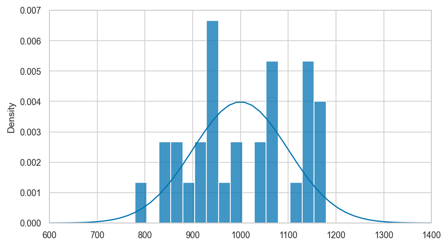
Clarification: empirical distribution of sample is not the same as \(f_N\)

# plot the pmf of uknown distritbuon f_N
from scipy.stats import norm
rvN = norm(1000, 100)
xs = np.linspace(600,1400)
ax = sns.lineplot(x=xs, y=rvN.pdf(xs))

# plot histogram from a single samples of size 30
sns.histplot(sample, binwidth=25, stat="density", ax=ax)
ax.set_xlim(600,1400)

(600.0, 1400.0)

# TODO: stem plot of sample
# TODO: stem plot alpha=0.1 of bsamples

Discussion

set random seed for repeatability

import random
random.seed(42)
random.random()

0.6394267984578837

import numpy as np
np.random.seed(43)
np.random.rand()

0.11505456638977896