Section 4.6 — Generalized linear models

Section 4.6 — Generalized linear models#

This notebook contains the code examples from Section 4.6 Generalized linear models from the No Bullshit Guide to Statistics.

Notebook setup#

# load Python modules
import os
import numpy as np
import pandas as pd
import seaborn as sns

# Figures setup
import matplotlib.pyplot as plt
plt.clf()  # needed otherwise `sns.set_theme` doesn't work
from plot_helpers import RCPARAMS
RCPARAMS.update({"figure.figsize": (5, 3)})   # good for screen
# RCPARAMS.update({'figure.figsize': (10, 3)})   # good for screen
# RCPARAMS.update({'figure.figsize': (4, 2)})  # good for print
sns.set_theme(
    context="paper",
    style="whitegrid",
    palette="colorblind",
    rc=RCPARAMS,
)

# High-resolution please
%config InlineBackend.figure_format = 'retina'

# Where to store figures
DESTDIR = "figures/lm/generalized"

<Figure size 640x480 with 0 Axes>

from ministats.utils import savefigure

#######################################################

Definitions#

Probability representations and link functions#

Odds#

0.5/(1-0.5), 0.9/(1-0.9), 0.2/(1-0.2)

(1.0, 9.000000000000002, 0.25)

Log-odds#

np.log(0.5/(1-0.5)), np.log(0.9/(1-0.9)), np.log(0.2/(1-0.2))

(0.0, 2.1972245773362196, -1.3862943611198906)

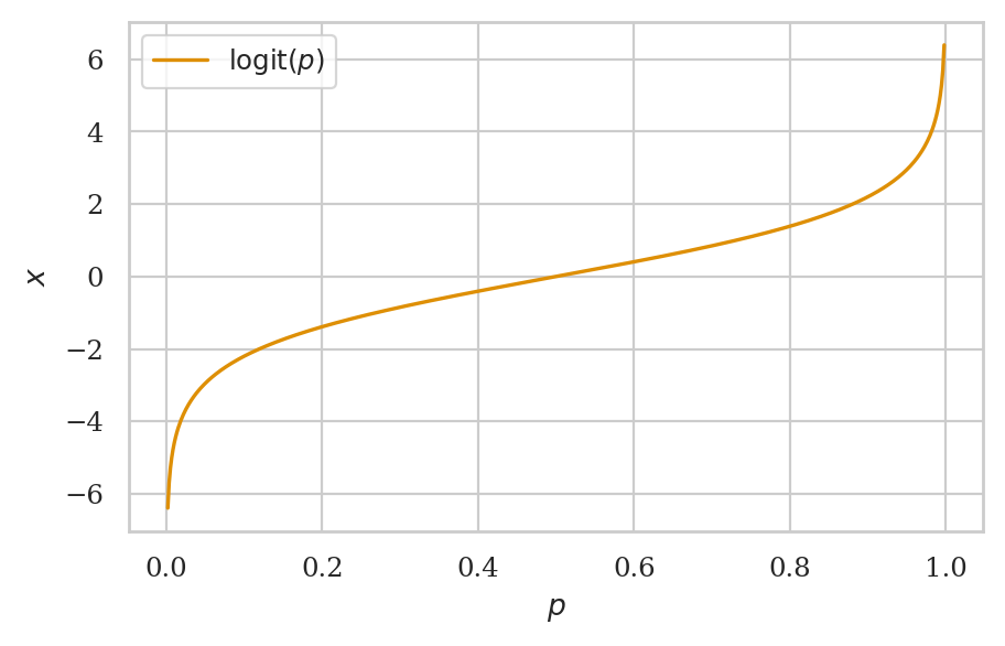
The logit function#

def logit(p):
    x = np.log(p / (1-p))
    return x

# ALT. import the function from `scipy.special`
from scipy.special import logit

logit(0.5), logit(0.9), logit(0.2)

(0.0, 2.1972245773362196, -1.3862943611198906)

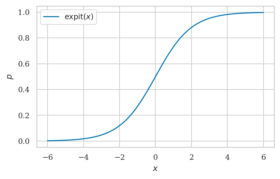
The logistic function#

def expit(x):
    p = 1 / (1 + np.exp(-x))
    return p

# ALT. import the function from `scipy.special`
from scipy.special import expit

expit(0), expit(2), expit(-2)

(0.5, 0.8807970779778823, 0.11920292202211755)

# FIGURES ONLY
fig, (ax1, ax2) = plt.subplots(1, 2, figsize=(6, 2))

# plot the expit function, a.k.a. the logistic function
xs = np.linspace(-6, 6, 500)
sns.lineplot(x=xs, y=expit(xs), ax=ax1, label="$\\mathrm{expit}(x)$")
ax1.set_xlabel("$x$")
ax1.set_ylabel("$p$")

# plot the logit function
ps = np.linspace(0, 1, 600)
sns.lineplot(x=ps, y=logit(ps), ax=ax2, label="$\\mathrm{logit}(p)$", color="C1")
ax2.set_xlabel("$p$")
ax2.set_ylabel("$x$")


filename = os.path.join(DESTDIR, "logistic_and_logit_functions.pdf")
savefigure(fig, filename, tight_layout_kwargs=dict(w_pad=3))

Saved figure to figures/lm/generalized/logistic_and_logit_functions.pdf

Saved figure to figures/lm/generalized/logistic_and_logit_functions.png

../_images/9c0a9fdd94a674e07b471a0540a9f1cd8c6a698d2f6d99ec86b7a21df307f1ae.png

The logistic and logit functions are inverses#

expit(logit(0.2))

0.2

logit(expit(3))

3.000000000000003

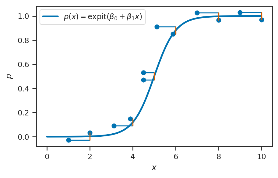
Logistic regression#

TODO FORMULA

# FIGURES ONLY
from scipy.stats import bernoulli
from scipy.special import expit

# Define the logistic regression model function
def expit_model(x):
    p = expit(-10 + 2*x)
    return p

xlims = [0, 10]

stem_half_width = 0.03

with sns.axes_style("ticks"):
    fig, ax = plt.subplots(figsize=(5, 3))

    # Plot the logistic regression model
    xs = np.linspace(xlims[0], xlims[1], 200)
    ps = expit_model(xs)
    sns.lineplot(x=xs, y=ps, ax=ax, label=r"$p(x) = \mathrm{expit}(\beta_0 + \beta_1x)$", linewidth=2)

    # Plot Bernoulli distributions at specified x positions
    x_positions = [2,4,5,6,8,10]
    for x_pos in x_positions:
        p_pos = expit_model(x_pos)
        ys = [0,1]
        pmf = bernoulli(p=p_pos).pmf(ys)
        ys_plot = [p_pos-stem_half_width, p_pos+stem_half_width]
        ax.stem(ys_plot, x_pos - pmf, bottom=x_pos, orientation='horizontal')

    # Figure setup
    ax.set_xlabel("$x$")
    ax.set_ylabel("$p$")
    ax.legend(loc="upper left")

    filename = os.path.join(DESTDIR, "logistic_regression_xy_with_stemplots.pdf")
    savefigure(fig, filename)

Saved figure to figures/lm/generalized/logistic_regression_xy_with_stemplots.pdf
Saved figure to figures/lm/generalized/logistic_regression_xy_with_stemplots.png

../_images/f8eb87760d167cbccafe0b3cfad3980f79bb440962f215d59d0adc049be0f3c8.png

expit(-6)

0.0024726231566347743

expit(10)

0.9999546021312976

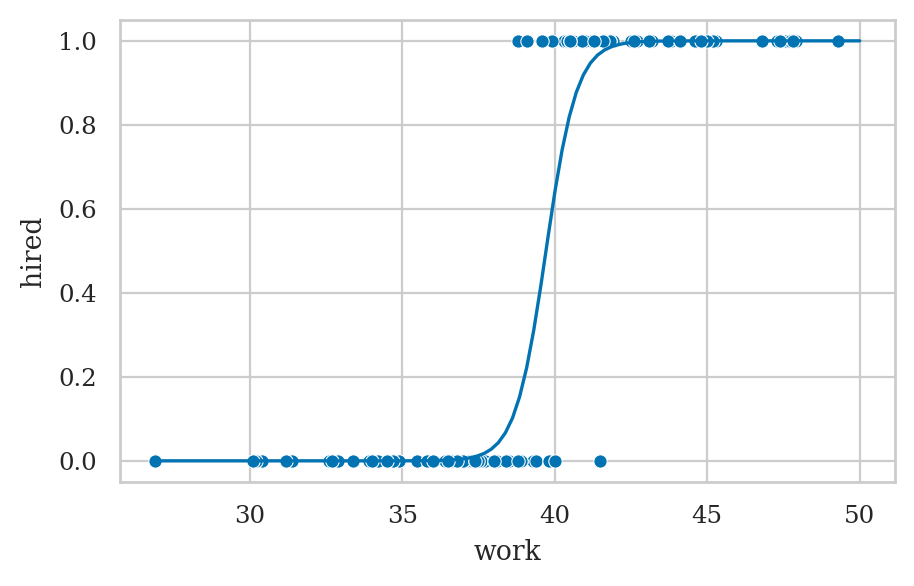
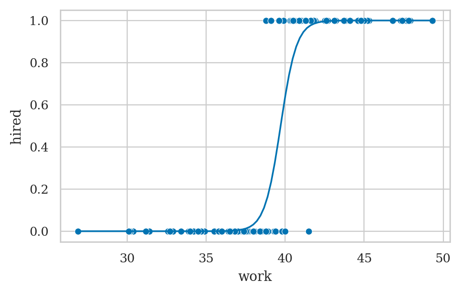
Example 1: hiring student interns#

interns = pd.read_csv("../datasets/interns.csv")
print(interns.shape)
interns.head(3)

(100, 2)

	work	hired
0	42.5	1
1	39.3	0
2	43.2	1

import statsmodels.formula.api as smf

lr1 = smf.logit("hired ~ 1 + work", data=interns).fit()
print(lr1.params)

Optimization terminated successfully.
         Current function value: 0.138101
         Iterations 10
Intercept   -78.693205
work          1.981458
dtype: float64

lr1.summary()

Logit Regression Results
Dep. Variable:	hired	No. Observations:	100
Model:	Logit	Df Residuals:	98
Method:	MLE	Df Model:	1
Date:	Fri, 18 Oct 2024	Pseudo R-squ.:	0.8005
Time:	20:56:31	Log-Likelihood:	-13.810
converged:	True	LL-Null:	-69.235
Covariance Type:	nonrobust	LLR p-value:	6.385e-26

	coef	std err	z	P>\|z\|	[0.025	0.975]
Intercept	-78.6932	19.851	-3.964	0.000	-117.600	-39.787
work	1.9815	0.500	3.959	0.000	1.001	2.962

Possibly complete quasi-separation: A fraction 0.32 of observations can be
perfectly predicted. This might indicate that there is complete
quasi-separation. In this case some parameters will not be identified.

ax = sns.scatterplot(data=interns, x="work", y="hired")
wgrid = np.linspace(27, 50, 100)
hired_preds = lr1.predict({"work": wgrid})
sns.lineplot(x=wgrid, y=hired_preds, ax=ax);

../_images/40d7b6f604a9e090773d10f418aeff050d9ee51beae5381c40fc4accdd06d156.png

from ministats import plot_reg
plot_reg(lr1)

# FIGURES ONLY
filename = os.path.join(DESTDIR, "logistic_regression_interns_hired_vs_work.pdf")
savefigure(plt.gcf(), filename)

Saved figure to figures/lm/generalized/logistic_regression_interns_hired_vs_work.pdf
Saved figure to figures/lm/generalized/logistic_regression_interns_hired_vs_work.png

../_images/b7d379e487c1762a21ef1840dab1ddf7a3d06f510511619208cd3edec7104d1d.png

lr1.summary()

Logit Regression Results
Dep. Variable:	hired	No. Observations:	100
Model:	Logit	Df Residuals:	98
Method:	MLE	Df Model:	1
Date:	Fri, 18 Oct 2024	Pseudo R-squ.:	0.8005
Time:	20:56:32	Log-Likelihood:	-13.810
converged:	True	LL-Null:	-69.235
Covariance Type:	nonrobust	LLR p-value:	6.385e-26

	coef	std err	z	P>\|z\|	[0.025	0.975]
Intercept	-78.6932	19.851	-3.964	0.000	-117.600	-39.787
work	1.9815	0.500	3.959	0.000	1.001	2.962

Possibly complete quasi-separation: A fraction 0.32 of observations can be
perfectly predicted. This might indicate that there is complete
quasi-separation. In this case some parameters will not be identified.

Interpreting the model parameters#

Parameters as changes in the log-odds#

lr1.params["work"]

1.9814577697476699

Parameters as ratios of odds#

np.exp(lr1.params["work"])

7.25330893626573

Differences in probabilities#

What is the marginal effect of the predictor work for an intern who invests 40 hours of effort?

# using `statsmodels`
lr1.get_margeff(atexog={1:40}).summary_frame()

	dy/dx	Std. Err.	z	Pr(>\|z\|)	Conf. Int. Low	Cont. Int. Hi.
work	0.45783	0.112623	4.065157	0.000048	0.237093	0.678567

lr1.get_margeff(atexog={1:42}).summary_frame()

	dy/dx	Std. Err.	z	Pr(>\|z\|)	Conf. Int. Low	Cont. Int. Hi.
work	0.020949	0.021358	0.98084	0.326672	-0.020912	0.06281

# # ALT. manual calculation plugging into derivative of `expit`
# p40 = lr1.predict({"work":40}).item()
# marg_effect_at_40 = p40 * (1 - p40) * lr1.params['work']
# marg_effect_at_40

Prediction#

p42 = lr1.predict({"work":42})[0]
p42

0.9893134055105761

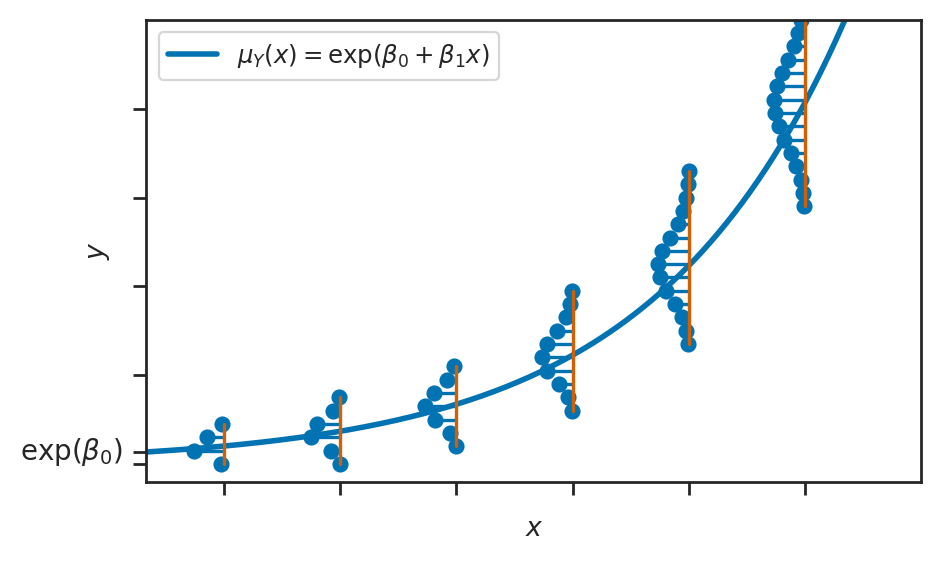
Poisson regression#

# FIGURES ONLY
from scipy.stats import poisson

# Define the linear model function
def exp_model(x):
    lam = np.exp(1 + 0.2*x)
    return lam

onepixel = 0.07

xlims = [0, 20]
ylims = [0, 100]

with sns.axes_style("ticks"):
    fig, ax = plt.subplots(figsize=(5, 3))

    # Plot the linear model
    xs = np.linspace(xlims[0], xlims[1], 200)
    lams = exp_model(xs)
    sns.lineplot(x=xs, y=lams, ax=ax, label=r"$\mu_Y(x) = \exp(\beta_0 + \beta_1x)$", linewidth=2)
    
    # Plot Gaussian distributions at specified x positions and add sigma lines
    x_positions = range(2, xlims[1]-1, 3)
    for x_pos in x_positions:
        lam_pos = exp_model(x_pos)
        sigma = np.sqrt(lam_pos)
        ys_lower = int(lam_pos-2.5*sigma)
        ys_upper = int(lam_pos+3.4*sigma)
        ys = np.arange(ys_lower, ys_upper, 3)
        pmf = poisson(mu=lam_pos).pmf(ys)
        # ax.fill_betweenx(ys, x_pos - 2 * pmf * sigma, x_pos, color="grey", alpha=0.5)
        ax.stem(ys, x_pos- 2 * pmf * sigma, bottom=x_pos, orientation='horizontal')
        # Draw vertical sigma line and label it on the opposite side of the Gaussian shape
        # ax.plot([x_pos+onepixel, x_pos+onepixel], [lam_pos, lam_pos - sigma], "k", lw=1)
        # ax.text(x_pos + 0.1, lam_pos - sigma / 2 - 3*onepixel, r"$\sigma$", fontsize=12, va="center")

    # y-intercept
    ax.text(0 - 0.6, np.exp(1), r"$\exp(\beta_0)$", fontsize=10, va="center", ha="right")

    # Set up x-axis
    ax.set_xlim(xlims)
    ax.set_xlabel("$x$")
    ax.set_xticks(range(2, xlims[1], 3))
    ax.set_xticklabels([])
    
    # Set up y-axis
    ax.set_ylim([ylims[0]-4,ylims[1]])
    ax.set_ylabel("$y$")
    ax.set_yticks(list(range(ylims[0],ylims[1],20)) + [np.exp(1)] )
    ax.set_yticklabels([])
    
    ax.legend(loc="upper left")

    filename = os.path.join(DESTDIR, "poisson_regression_xy_with_stemplots.pdf")
    savefigure(fig, filename)

Saved figure to figures/lm/generalized/poisson_regression_xy_with_stemplots.pdf
Saved figure to figures/lm/generalized/poisson_regression_xy_with_stemplots.png

../_images/f6f90f0bfe6e5c1a9426f29489e785999e88ff3e175e7a39492521e73f3932bc.png

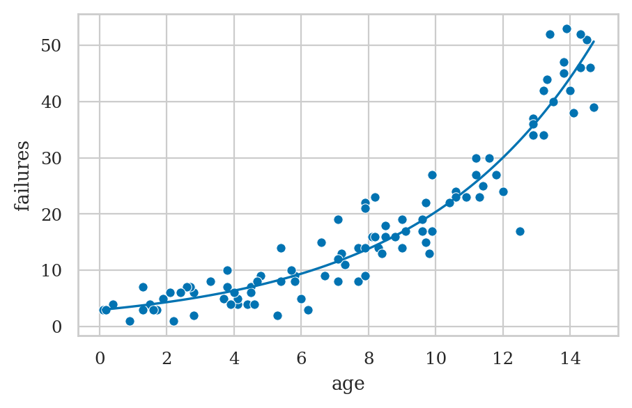
Example 2: hard disk failures over time#

hdisks = pd.read_csv("../datasets/hdisks.csv")
hdisks.head(3)

	age	failures
0	1.7	3
1	14.6	46
2	10.9	23

import statsmodels.formula.api as smf

pr2 = smf.poisson("failures ~ 1 + age", data=hdisks).fit()
pr2.params

Optimization terminated successfully.
         Current function value: 2.693129
         Iterations 6

Intercept    1.075999
age          0.193828
dtype: float64

pr2.summary()

Poisson Regression Results
Dep. Variable:	failures	No. Observations:	100
Model:	Poisson	Df Residuals:	98
Method:	MLE	Df Model:	1
Date:	Fri, 18 Oct 2024	Pseudo R-squ.:	0.6412
Time:	20:56:32	Log-Likelihood:	-269.31
converged:	True	LL-Null:	-750.68
Covariance Type:	nonrobust	LLR p-value:	2.271e-211

	coef	std err	z	P>\|z\|	[0.025	0.975]
Intercept	1.0760	0.076	14.114	0.000	0.927	1.225
age	0.1938	0.007	28.603	0.000	0.181	0.207

from ministats import plot_reg
plot_reg(pr2)

# FIGURES ONLY
filename = os.path.join(DESTDIR, "poisson_regression_hdisks_failures_vs_age.pdf")
savefigure(plt.gcf(), filename)

Saved figure to figures/lm/generalized/poisson_regression_hdisks_failures_vs_age.pdf
Saved figure to figures/lm/generalized/poisson_regression_hdisks_failures_vs_age.png

../_images/fbc79b4542c0a6427d1d42163acad0029218b993c0dd40190c75dae5d0b64f88.png

pr2.summary()

Poisson Regression Results
Dep. Variable:	failures	No. Observations:	100
Model:	Poisson	Df Residuals:	98
Method:	MLE	Df Model:	1
Date:	Fri, 18 Oct 2024	Pseudo R-squ.:	0.6412
Time:	20:56:33	Log-Likelihood:	-269.31
converged:	True	LL-Null:	-750.68
Covariance Type:	nonrobust	LLR p-value:	2.271e-211

	coef	std err	z	P>\|z\|	[0.025	0.975]
Intercept	1.0760	0.076	14.114	0.000	0.927	1.225
age	0.1938	0.007	28.603	0.000	0.181	0.207

Interpreting the model parameters#

Log-counts#

pr2.params["age"]

0.19382784821454072

Incidence rate ratio (IRR)#

np.exp(pr2.params["age"])

1.213887292102993

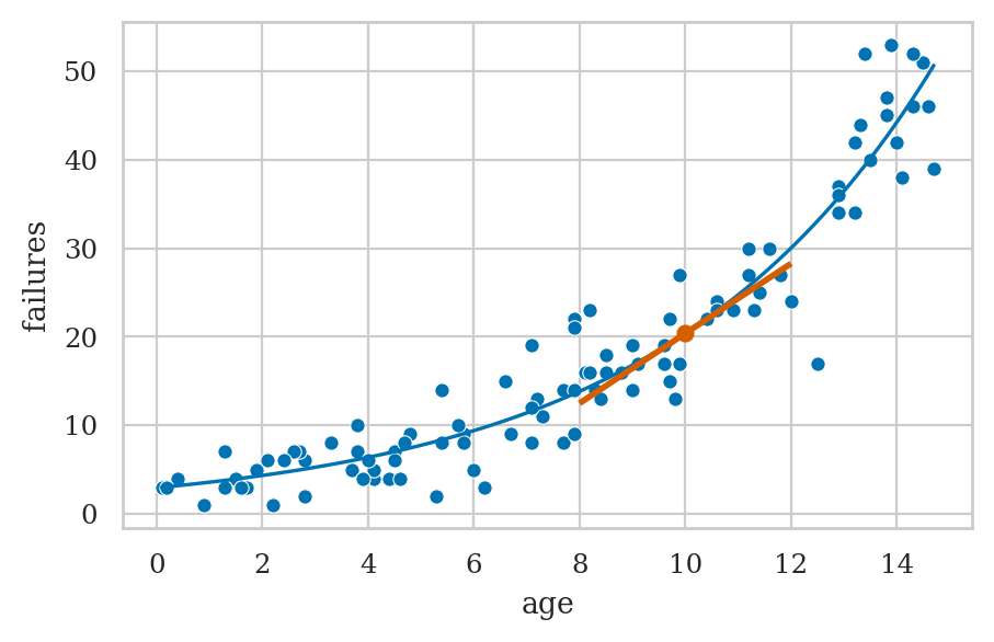
Marginal effect#

What is the marginal effect of the predictor age for a 10 year old hard disk installation?

# using `statsmodels` .get_margeff() method
pr2.get_margeff(atexog={1:10}).summary_frame()

	dy/dx	Std. Err.	z	Pr(>\|z\|)	Conf. Int. Low	Cont. Int. Hi.
age	3.94912	0.151882	26.001165	4.804151e-149	3.651435	4.246804

# # ALT. manual calculation of the slope by evaluating the derivative
# b_0 = pr2.params['Intercept']
# b_age = pr2.params['age']
# np.exp(b_0 + b_age*10)*b_age

ax = plot_reg(pr2)

# Show the tangent line at age=10 (the marginal effect)
ptx, pty = (10, pr2.predict({"age":10})[0])
slope = pr2.get_margeff(atexog={1:10}).margeff[0]
dx = 2
endpoint1 = [ptx - dx, pty - dx*slope]
endpoint2 = [ptx + dx, pty + dx*slope]
lines = [[endpoint1, endpoint2]]
from matplotlib import collections as mc
lc = mc.LineCollection(lines, color="r", lw=2)
ax.plot([ptx], [pty], marker="o", color="r", alpha=1)
ax.add_collection(lc);

../_images/8c81ddfe471ef14d948e44279b0159342c317fea6893b10a141f2f6d95361231.png

Predictions#

lam10 = pr2.predict({"age":10})[0]
lam10

20.374365915173986

from scipy.stats import poisson
Hhat = poisson(mu=lam10)
Hhat.ppf(0.05), Hhat.ppf(0.95)

(13.0, 28.0)

Explanations#

The exponential family of distributions#

exponential
Gaussian (normal)
Poisson
Binomial

The generalized linear model template#

choose

Generalized linear models using statsmodels#

import statsmodels.api as sm

Norm = sm.families.Gaussian()
Bin = sm.families.Binomial()
Pois = sm.families.Poisson()

Linear model#

students = pd.read_csv('../datasets/students.csv')
formula0 = "score ~ 1 + effort"
glm0 = smf.glm(formula0, data=students, family=Norm).fit()
glm0.params

Intercept    32.465809
effort        4.504850
dtype: float64

Logistic regression#

formula1 = "hired ~ 1 + work"
glm1 = smf.glm(formula1, data=interns, family=Bin).fit()
glm1.params
# glm1.summary()

Intercept   -78.693205
work          1.981458
dtype: float64

Poisson regression#

formula2 = "failures ~ 1 + age"
glm2 = smf.glm(formula2, data=hdisks, family=Pois).fit()
glm2.params
# glm2.summary()

Intercept    1.075999
age          0.193828
dtype: float64

Fitting generalized linear models#

Discussion#

Model diagnostics and validation#

# Dispersion from GLM attributes
# glm2.pearson_chi2 / glm2.df_resid

# Calculate Pearson chi-squared statistic
observed = hdisks['failures']
predicted = pr2.predict()
pearson_residuals = (observed - predicted) / np.sqrt(predicted)
pearson_chi2 = np.sum(pearson_residuals**2)
df_resid = pr2.df_resid
dispersion = pearson_chi2 / df_resid
print(f'Dispersion: {dispersion}')
# If dispersion > 1, consider Negative Binomial regression

Dispersion: 0.9869289289681199

Logistic regression as a building blocks for neural networks#

The operation of the perceptron, which is the basic building block of neural networks, is essentially the same as linear regression model:

constant intercept (bias term)
linear combination of inputs
nonlinear function used to force the output to be between 0 and 1

Limitations of GLMs#

GLMs assume observations are independent
Assumes distribution \(\mathcal{M}\) is one of the exponential family
Outliers can be problematic
Interpretability

Exercises#

Exercise 1: probabilities to odds and log-odds#

0.3/(1-0.3), 0.99/(1-0.99), 0.7/(1-0.7)

(0.4285714285714286, 98.99999999999991, 2.333333333333333)

logit(0.3), logit(0.99), logit(0.7)

(-0.8472978603872036, 4.595119850134589, 0.8472978603872034)

Exercise 2: log-odds to probabilities#

expit(-1), expit(1), expit(2)

(0.2689414213699951, 0.7310585786300049, 0.8807970779778823)

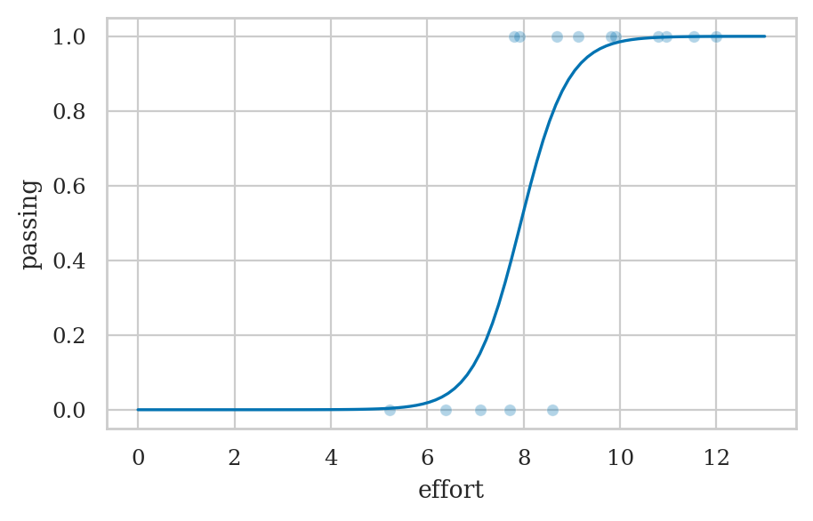
Exercise 3: students pass or fail#

a) Load the dataset students.csv and add a column passing that contains 1 or 0, based on the above threshold score of 70.

students = pd.read_csv('../datasets/students.csv')
students["passing"] = (students["score"] > 70).astype(int)
# students.head()

b) Fit a logistic regression model for passing based on effort variable.

lmpass = smf.logit("passing ~ 1 + effort", data=students).fit()
print(lmpass.params)

efforts = np.linspace(0, 13, 100)
passing_preds = lmpass.predict({"effort": efforts})
ax = sns.scatterplot(data=students, x="effort", y="passing", alpha=0.3)
sns.lineplot(x=efforts, y=passing_preds, ax=ax);

filename = os.path.join(DESTDIR, "logistic_regression_students_passing_vs_effort.pdf")
savefigure(plt.gcf(), filename)

Optimization terminated successfully.
         Current function value: 0.276583
         Iterations 8
Intercept   -16.257302
effort        2.047882
dtype: float64

Saved figure to figures/lm/generalized/logistic_regression_students_passing_vs_effort.pdf
Saved figure to figures/lm/generalized/logistic_regression_students_passing_vs_effort.png

../_images/349eeef3ca53530063f48a4aa6529fd6cac023d01a6da7cc79829a484bda0066.png

c) Use your model to predict the probability of a new student with effort 10 will pass.

lmpass.predict({"effort":10})

0    0.985536
dtype: float64

# ALT. compute prediction manually
intercept, b_effort = lmpass.params
expit(intercept + b_effort*10)

0.9855358765361845

Exercise 4: titanic survival data#

Fit a logistic regression model that calculates the probability of survival for people who were on the Titanic, based on the data in datasets/exercises/titanic.csv. Use the variables age, sex, and pclass as predictors.

cf. Titanic_Logistic_Regression.ipynb

titanic = pd.read_csv('../datasets/exercises/titanic.csv')
formula = "survived ~ age + C(sex) + C(pclass)"
lrtitanic = smf.logit(formula, data=titanic).fit()
lrtitanic.params

Optimization terminated successfully.
         Current function value: 0.453279
         Iterations 6

Intercept         3.777013
C(sex)[T.M]      -2.522781
C(pclass)[T.2]   -1.309799
C(pclass)[T.3]   -2.580625
age              -0.036985
dtype: float64

Use your logistic regression model to estimate the probability of survival for a 30 year old female traveling in second class.

pass30Fpclass2 = {"age":30, "sex":"F", "pclass":2}
lrtitanic.predict(pass30Fpclass2)

0    0.795378
dtype: float64

# # Cross check with sklearn
# from sklearn.linear_model import LogisticRegression
# df = pd.get_dummies(titanic, columns=['sex', 'pclass'], drop_first=True)
# X, y = df.drop('survived', axis=1), df['survived']
# sktitanic = LogisticRegression(penalty=None)
# sktitanic.fit(X, y)
# sktitanic.intercept_, sktitanic.coef_

Exercise 5: asthma attacks#

Fit a Poisson regression model to the ../datasets/exercises/asthma.csv dataset.

data source drkamarul/multivar_data_analysis

asthma = pd.read_csv("../datasets/exercises/asthma.csv")
asthma

	gender	res_inf	ghq12	attack
0	female	yes	21	6
1	male	no	17	4
2	male	yes	30	8
3	female	yes	22	5
4	male	yes	27	2
...	...	...	...	...
115	male	yes	0	2
116	female	yes	31	2
117	female	yes	18	2
118	female	yes	21	3
119	female	yes	11	2

120 rows × 4 columns

formula_asthma = "attack ~ 1 + C(gender) + C(res_inf) + ghq12"
prasthma = smf.poisson(formula_asthma, data=asthma).fit()
prasthma.params

Optimization terminated successfully.
         Current function value: 1.707281
         Iterations 6

Intercept           -0.315387
C(gender)[T.male]   -0.041905
C(res_inf)[T.yes]    0.426431
ghq12                0.049508
dtype: float64

cf. https://bookdown.org/drki_musa/dataanalysis/poisson-regression.html#multivariable-analysis-1

Exercise 6: student admissions dataset#

The dataset datasets/exercises/binary.csv contains information about the acceptance decision for 400 students to a prestigious school. Try to fit a logistic regression model for the variable admit using the variables gre, gpa, and rank as predictors.

# ORIGINAL https://stats.idre.ucla.edu/stat/data/binary.csv
binary = pd.read_csv('../datasets/exercises/binary.csv')
binary.head(3)

	admit	gre	gpa	rank
0	0	380	3.61	3
1	1	660	3.67	3
2	1	800	4.00	1

lrbinary = smf.logit('admit ~ gre + gpa + C(rank)', data=binary).fit()
lrbinary.params

Optimization terminated successfully.
         Current function value: 0.573147
         Iterations 6

Intercept      -3.989979
C(rank)[T.2]   -0.675443
C(rank)[T.3]   -1.340204
C(rank)[T.4]   -1.551464
gre             0.002264
gpa             0.804038
dtype: float64

The above model uses the rank=1 as the reference category an the log odds reported are with respect to this catrgory

\[ \log p(accept|rank=1) / \log p(accept|rank=2) = \texttt{C(rank)rank[T.2]} = -0.675443 \]

etc. for others rank[T.3] -1.340204 rank[T.4] -1.551464

See LogisticRegressionChangeOfReferenceCategoricalValue.ipynb for exercise recodign relative to different refrence level.

# # Cross check with sklearn
# from sklearn.linear_model import LogisticRegression
# df = pd.get_dummies(binary, columns=['rank'], drop_first=True)
# X, y = df.drop("admit", axis=1), df["admit"]
# lr = LogisticRegression(solver="lbfgs", penalty=None, max_iter=1000)
# lr.fit(X, y)
# lr.intercept_,  lr.coef_

Exercise 7: ship accidents#

https://rdrr.io/cran/AER/man/ShipAccidents.html

https://pages.stern.nyu.edu/~wgreene/Text/tables/tablelist5.htm

https://pages.stern.nyu.edu/~wgreene/Text/tables/TableF21-3.txt

# TODO

Bonus Exercises#

Bonus exercise A: honors class#

https://stats.oarc.ucla.edu/other/mult-pkg/faq/general/faq-how-do-i-interpret-odds-ratios-in-logistic-regression/

honors = pd.read_csv("../datasets/exercises/honors.csv")
honors.sample(4)

	female	read	write	math	hon	femalexmath
76	0	55	61	54	1	0
116	1	43	54	55	0	55
80	0	63	59	57	0	0
55	0	39	39	44	0	0

Constant model#

lrhon1 = smf.logit("hon ~ 1", data=honors).fit()
lrhon1.params

Optimization terminated successfully.
         Current function value: 0.556775
         Iterations 5

Intercept   -1.12546
dtype: float64

expit(lrhon1.params["Intercept"])

0.24500000000000005

honors["hon"].value_counts(normalize=True)

hon
0    0.755
1    0.245
Name: proportion, dtype: float64

Using only a categorical variable#

lrhon2 = smf.logit("hon ~ 1 + female", data=honors).fit()
lrhon2.params

Optimization terminated successfully.
         Current function value: 0.549016
         Iterations 5

Intercept   -1.470852
female       0.592782
dtype: float64

pd.crosstab(honors["hon"], honors["female"], margins=True)

female	0	1	All
hon
0	74	77	151
1	17	32	49
All	91	109	200

b0 = lrhon2.params["Intercept"]
b_female = lrhon2.params["female"]

# male prob
expit(b0), 17/91

(0.18681318681318684, 0.18681318681318682)

# male odds
np.exp(b0), 17/74  # = (17/91) / (74/91)

(0.2297297297297298, 0.22972972972972974)

# male log-odds
b0, np.log(17/74)

(-1.4708517491479534, -1.4708517491479536)

# female prob
expit(b0 + b_female), 32/109

(0.2935779816513761, 0.29357798165137616)

# female odds
np.exp(b0 + b_female), 32/77 # = (32/109) / (77/109)

(0.4155844155844155, 0.4155844155844156)

b0 + b_female, np.log(32/77)

(-0.8780695190539575, -0.8780695190539572)

# odds female relative to male
np.exp(b_female)

1.809014514896867

Logistic regression with a single continuous predictor variable#

lrhon3 = smf.logit("hon ~ 1 + math", data=honors).fit()
lrhon3.params

Optimization terminated successfully.
         Current function value: 0.417683
         Iterations 7

Intercept   -9.793942
math         0.156340
dtype: float64

So the model equation is

\[ \log(p/(1-p)) = \texttt{logit}(p) = -9.793942 + .1563404 \cdot \texttt{math} \]

# Increase in log-odds between math=54 and math=55
p54 = lrhon3.predict({"math":[54]}).item()
p55 = lrhon3.predict({"math":[55]}).item()
logit(p55) - logit(p54), lrhon3.params["math"]

(0.1563403555859233, 0.15634035558592282)

We can say now that the coefficient for math is the difference in the log odds. In other words, for a one-unit increase in the math score, the expected change in log odds is .1563404.

# Increase (multiplicative) in odds for unit increase in math
np.exp(lrhon3.params["math"]),  (p55/(1-p55)) / (p54/(1-p54))

(1.1692240873242836, 1.1692240873242843)

So we can say for a one-unit increase in math score, we expect to see about 17% increase in the odds of being in an honors class. This 17% of increase does not depend on the value that math is held at.

Logistic regression with multiple predictor variables and no interaction terms#

lrhon4 = smf.logit("hon ~ 1 + math + female + read", data=honors).fit()
lrhon4.params

Optimization terminated successfully.
         Current function value: 0.390424
         Iterations 7

Intercept   -11.770246
math          0.122959
female        0.979948
read          0.059063
dtype: float64

Logistic regression with an interaction term of two predictor variables#

lrhon5 = smf.logit("hon ~ 1 + math + female + femalexmath", data=honors).fit()
lrhon5.params

Optimization terminated successfully.
         Current function value: 0.399417
         Iterations 7

Intercept     -8.745841
math           0.129378
female        -2.899863
femalexmath    0.066995
dtype: float64

# ALT. without using `femalexmath` column
# lrhon5 = smf.logit("hon ~ 1 + math + female + female*math", data=honors).fit()
# lrhon5.params

Bonus exercise: LA high schools (NOT A VERY GOOD FIT FOR POISSON MODEL)#

Dataset info: http://www.philender.com/courses/intro/assign/data.html

This dataset consists of data from computer exercises collected from two high school in the Los Angeles area.

http://www.philender.com/courses/intro/code.html

lahigh_raw = pd.read_stata("https://stats.idre.ucla.edu/stat/stata/notes/lahigh.dta")
lahigh = lahigh_raw.convert_dtypes()

lahigh["gender"] = lahigh["gender"].astype(object).replace({1:"F", 2:"M"})
lahigh["ethnic"] = lahigh["ethnic"].astype(object).replace({
    1:"Native American",
    2:"Asian",
    3:"African-American",
    4:"Hispanic",
    5:"White",
    6:"Filipino",
    7:"Pacific Islander"})
lahigh["school"] = lahigh["school"].astype(object).replace({1:"Alpha", 2:"Beta"})
lahigh.head()

	id	gender	ethnic	school	mathpr	langpr	mathnce	langnce	biling	daysabs
0	1001	M	Hispanic	Alpha	63	36	56.988831	42.450859	2	4
1	1002	M	Hispanic	Alpha	27	44	37.094158	46.820587	2	4
2	1003	F	Hispanic	Alpha	20	38	32.275455	43.566574	2	2
3	1004	F	Hispanic	Alpha	16	38	29.056717	43.566574	2	3
4	1005	F	Hispanic	Alpha	2	14	6.748048	27.248474	3	3

formula = "daysabs ~ 1 + mathnce + langnce + C(gender)"
prlahigh = smf.poisson(formula, data=lahigh).fit()
prlahigh.params

Optimization terminated successfully.
         Current function value: 4.898642
         Iterations 5

Intercept         2.687666
C(gender)[T.M]   -0.400921
mathnce          -0.003523
langnce          -0.012152
dtype: float64

# IRR
np.exp(prlahigh.params[1:])

C(gender)[T.M]    0.669703
mathnce           0.996483
langnce           0.987921
dtype: float64

# CI for IRR F 
np.exp(prlahigh.conf_int().loc["C(gender)[T.M]"])

0    0.609079
1    0.736361
Name: C(gender)[T.M], dtype: float64

# prlahigh.summary()
# prlahigh.aic, prlahigh.bic

Diagnostics#

via https://www.statsmodels.org/dev/examples/notebooks/generated/postestimation_poisson.html

prdiag = prlahigh.get_diagnostic()
# Plot observed versus predicted frequencies for entire sample
# prdiag.plot_probs();

# Other:
# ['plot_probs',
#  'probs_predicted',
#  'results',
#  'test_chisquare_prob',
#  'test_dispersion',
#  'test_poisson_zeroinflation',
#  'y_max']

# Code to get exactly the same numbers as in
# https://stats.oarc.ucla.edu/stata/output/poisson-regression/  
formula2 = "daysabs ~ 1 + mathnce + langnce + C(gender, Treatment(1))"
prlahigh2 = smf.poisson(formula2, data=lahigh).fit()
prlahigh2.params

Optimization terminated successfully.
         Current function value: 4.898642
         Iterations 5

Intercept                       2.286745
C(gender, Treatment(1))[T.F]    0.400921
mathnce                        -0.003523
langnce                        -0.012152
dtype: float64

Links#

TODO

Section 4.6 — Generalized linear models

Contents

Section 4.6 — Generalized linear models#

Notebook setup#

Definitions#

Probability representations and link functions#

Odds#

Log-odds#

The logit function#

The logistic function#

The logistic and logit functions are inverses#

Logistic regression#

Example 1: hiring student interns#

Interpreting the model parameters#

Parameters as changes in the log-odds#

Parameters as ratios of odds#

Differences in probabilities#

Prediction#

Poisson regression#

Example 2: hard disk failures over time#

Interpreting the model parameters#

Log-counts#

Incidence rate ratio (IRR)#

Marginal effect#

Predictions#

Explanations#

The exponential family of distributions#

The generalized linear model template#

Generalized linear models using statsmodels#

Linear model#

Logistic regression#

Poisson regression#

Fitting generalized linear models#

Discussion#

Model diagnostics and validation#

Logistic regression as a building blocks for neural networks#

Limitations of GLMs#

Exercises#

Exercise 1: probabilities to odds and log-odds#

Exercise 2: log-odds to probabilities#

Exercise 3: students pass or fail#

Exercise 4: titanic survival data#

Exercise 5: asthma attacks#

Exercise 6: student admissions dataset#

Exercise 7: ship accidents#

Bonus Exercises#

Bonus exercise A: honors class#

Constant model#

Using only a categorical variable#

Logistic regression with a single continuous predictor variable#

Logistic regression with multiple predictor variables and no interaction terms#

Logistic regression with an interaction term of two predictor variables#

Bonus exercise: LA high schools (NOT A VERY GOOD FIT FOR POISSON MODEL)#

Diagnostics#

Links#