Section 2.4 — Continuous random variables#
This notebook contains all the code examples from Section 2.4 Continuous random variables of the No Bullshit Guide to Statistics.
Notebook setup#
We’ll start by importing the Python modules we’ll need for this notebook.
# Ensure required Python modules are installed
%pip install --quiet numpy scipy seaborn ministats
Note: you may need to restart the kernel to use updated packages.
# Load Python modules
import numpy as np
import seaborn as sns
import matplotlib.pyplot as plt
# Figures setup
sns.set_theme(
    context="paper",
    style="whitegrid",
    palette="colorblind",
    rc={"font.family": "serif",
        "font.serif": ["Palatino", "DejaVu Serif", "serif"],
        "figure.figsize": (7.5, 2.3)},
)
%config InlineBackend.figure_format = 'retina'
# Simple float __repr__
import numpy as np
if int(np.__version__.split(".")[0]) >= 2:
    np.set_printoptions(legacy='1.25')
Definitions#
Random variables#
random variable \(X\): a quantity that can take on different values.
sample space \(\mathcal{X}\): describes the set of all possible outcomes of the random variable \(X\).
outcome: a particular value \(\{X = x\}\) that can occur as a result of observing the random variable \(X\).
event subset of the sample space \(\{a \leq X \leq b\}\) that can occur as a result of observing the random variable \(X\).
\(f_X\): the probability density function (PDF) is a function that assigns probabilities to the different outcome in the sample space of a random variable. The probability distribution function of the random variable \(X\) is a function of the form \(f_X: \mathcal{X} \to \mathbb{R}\).
Calculus prerequisites#
Functions#
In Python, we define functions using the def keyword.
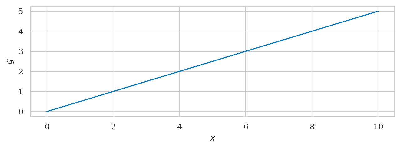
For example, the code cell below defines the function \(g(x)=\frac{1}{2}x\),
then evaluate it on the input \(x=5\).
# define the function g that takes input x
def g(x):
    return 0.5 * x

# calling the function g on input x=5
g(5)
2.5
xs = np.linspace(0, 10, 1000)
gs = g(xs)

ax = sns.lineplot(x=xs, y=gs)
ax.set_xlabel("$x$")
ax.set_ylabel("$g$");
Integrals#
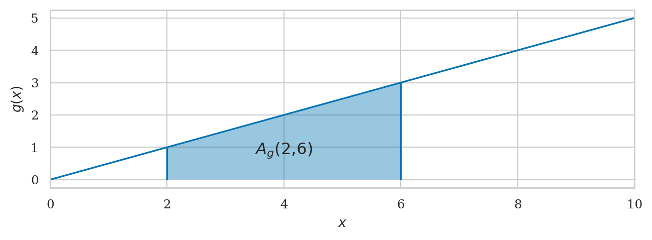
The area under the graph of the function \(g\), between \(x=2\) and \(x=6\) is calculated using the following integral:
from ministats.calculus import plot_integral

# limits of integration
a = 2
b = 6

# highlight the area under g(x) between x=a and x=b
plot_integral(g, a=a, b=b, xlim=[0,10], flabel="g", autolabel=True);
The function quad from the scipy.integrate module
allows us to compute the integral of any function.
from scipy.integrate import quad
quad(g, a=2, b=6)
(8.0, 8.881784197001252e-14)
The function quad returns two numbers as output:
\(\big(A_g(2,6),\epsilon\big)\).
The first number is the value of the area we’re interested in.
The second number,
\(\epsilon\),
indicates the accuracy of the procedure used to calculate the area,
which is \(\epsilon=8.88\times 10^{-14}\) in this case.
We’re usually only interested in the value of the area,
so we select the first element of the output,
as shown below.
quad(g, a=2, b=6)[0]
8.0
We used [0] to select the first value of the output,
which is the value of the area \(A_g(2,6)=8\).
Integral functions#
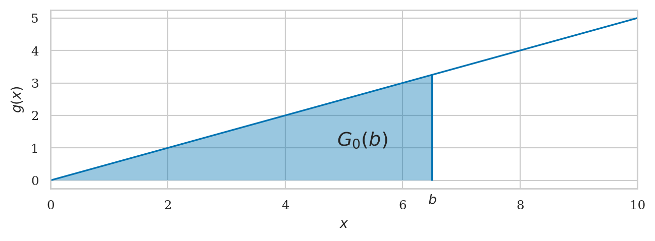
The integral function \(F_0(b)\) corresponds to the area calculation with a variable upper limit of integration \(A_f(0,b)\). It is defined as:
The integral function of the function \(g(x)=\frac{1}{2}x\) is \(G_0(b) = A_g(0,b) = \frac{1}{4}x^2\).
b = 6.5
ax = plot_integral(g, a=0, b=b, xlim=[0,10], flabel="g")
ax.text(3*b/4, g(b)/3, "$G_0(b)$", fontsize="x-large")
ax.text(b, -0.4, "$b$", ha="center", va="top");
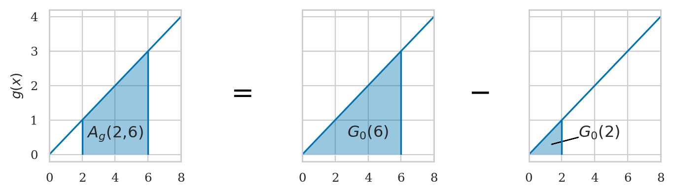
from ministats.book.figures import integral_as_difference_in_G

integral_as_difference_in_G();
Computer models for random variables#
Consider the computer model rvX for the random variable \(X \sim \mathcal{M}(\theta)\).
We saw previously in Section 2.1
TODO: compare and sync with text with Section 2.1
<model>: the family of probability distributions<params>: parameters of the model—specific value of the control knobs we choose in the general family of distributions to create a particular distribution<model>(<params>): a particular instance of probability model created by choosing a model family<model>and the model parameters<params>.example 1: uniform family of distribution \(\mathcal{U}(\alpha,\beta)\) with parameters \(\alpha\) and \(\beta\).
example 2: normal family of distribution \(\mathcal{N}(\mu,\sigma)\) with parameters \(\mu\) and \(\sigma\).
\(\sim\): math shorthand symbol that stands for “is distributed according to.” For example \(X \sim \texttt{model}(\theta)\) means the random variable \(X\) is distributed according to model instance \(\texttt{model}\) and parameters \(\theta\).
Summary of methods#
TODO: import table of methods
Examples#
The continuous uniform family of distribution \(\mathcal{U}(\alpha,\beta)\), which assigns equal probabilities to all outcomes in the interval \([\alpha,\beta]\). To create a computer model for a continuous uniform distribution \(\mathcal{U}(\alpha,\beta)\), use the code
uniform(loc=alpha,scale=beta-alpha).Normal distribution \(\mathcal{N}(\mu,\sigma)\) …
Example 1: uniform distribution#
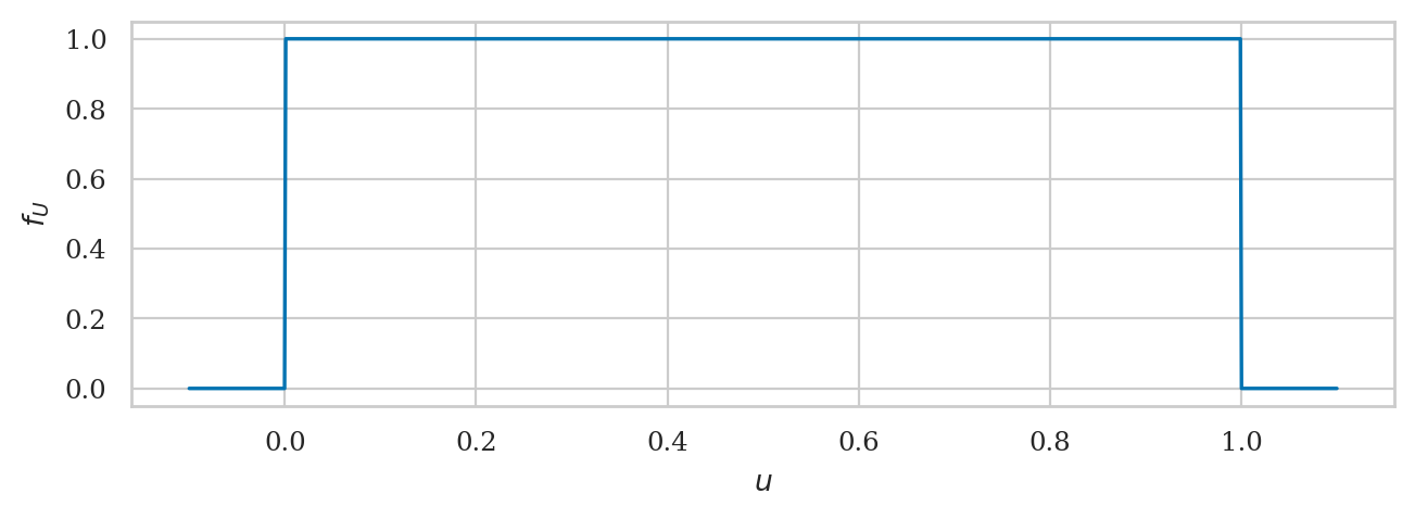
The uniform distribution \(U \sim \mathcal{U}(0,1)\) is described by the following probability density function:
For a uniform distribution \(\mathcal{U}(0,1)\), each \(u\) between 0 and 1 is equally likely to occur, and values of \(u\) outside this range have zero probability of occurring.
# define the computer model `rvU` for the random variable U
from scipy.stats import uniform
alpha = 0
beta = 1
rvU = uniform(loc=alpha, scale=beta-alpha)
Plotting the uniform probability density function#
us = np.linspace(-0.1, 1.1, 1000)
fUs = rvU.pdf(us)
ax = sns.lineplot(x=us, y=fUs)
ax.set_xlabel("$u$")
ax.set_ylabel("$f_U$");
Alternatively,
we can use the helper function plot_pdf from the ministats library
to plot the PDF \(f_U\).
%pip install -q ministats
Note: you may need to restart the kernel to use updated packages.
from ministats import plot_pdf
plot_pdf(rvU, xlims=[-0.1, 1.1], rv_name="U");
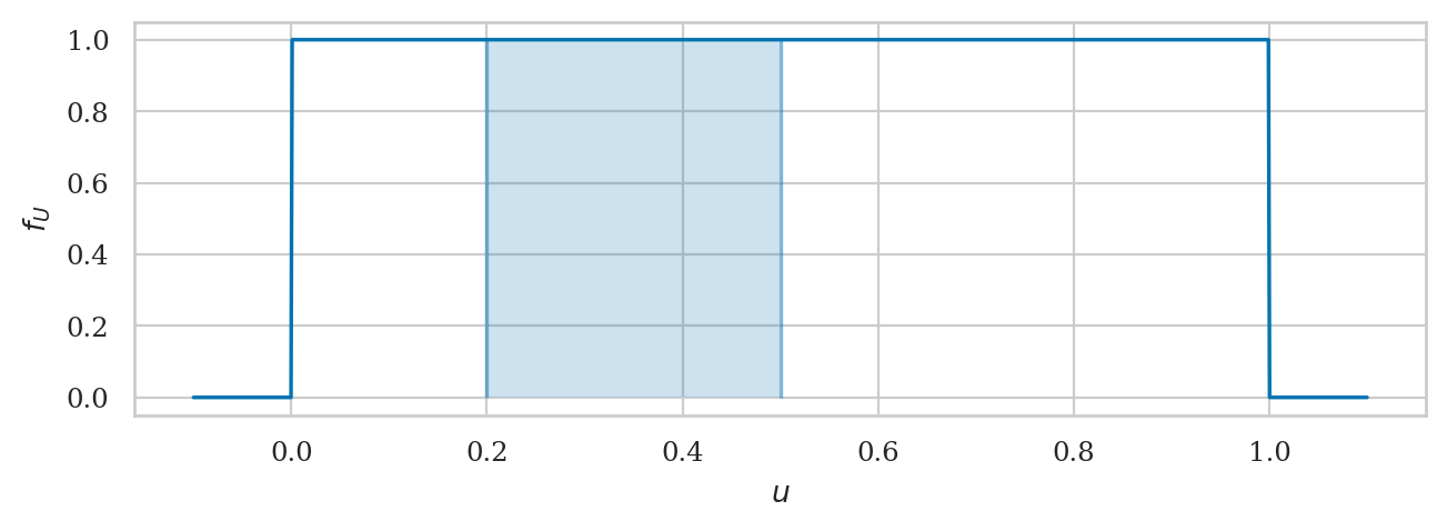
We can pass the options a and b to the function plot_pdf
to highlight the area that corresponds to
the probability of the event \(\{ \texttt{a} \leq U \leq \texttt{b} \}\).
plot_pdf(rvU, xlims=[-0.1, 1.1], rv_name="U", a=0.2, b=0.5);
Calculating the probability of an event#
TODO: math
# use `quad` function to integrate rvU.pdf between 0.2 and 0.5
from scipy.integrate import quad
quad(rvU.pdf, a=0.2, b=0.5)[0]
0.3
The total area under the graph of \(f_U\) is equal to \(1\).
quad(rvU.pdf, a=0, b=1)[0]
1.0
Example 2: standard normal distribution#
A standard normal random variable \(Z \sim \mathcal{N}(\mu=0,\sigma=1)\) is described by the probability density function:
The mean \(\mu_Z=0\) (the Greek letter mu) and the standard deviation \(\sigma_Z=1\) (the Greek letter sigma) are called the parameters of the distribution.
The math notation \(\mathcal{N}(\mu, \sigma)\) is used to describe the whole family of normal probability distributions, and \(Z \sim \mathcal{N}(\mu_Z=0, \sigma_Z=1)\) is a particular instance of the distribution with mean \(\mu_Z = 0\) and standard deviation \(\sigma_Z = 1\).
# define the computer model `rvZ` for the random variable Z
from scipy.stats import norm
muZ = 0
sigmaZ = 1
rvZ = norm(muZ, sigmaZ)
Plotting the normal probability density function#
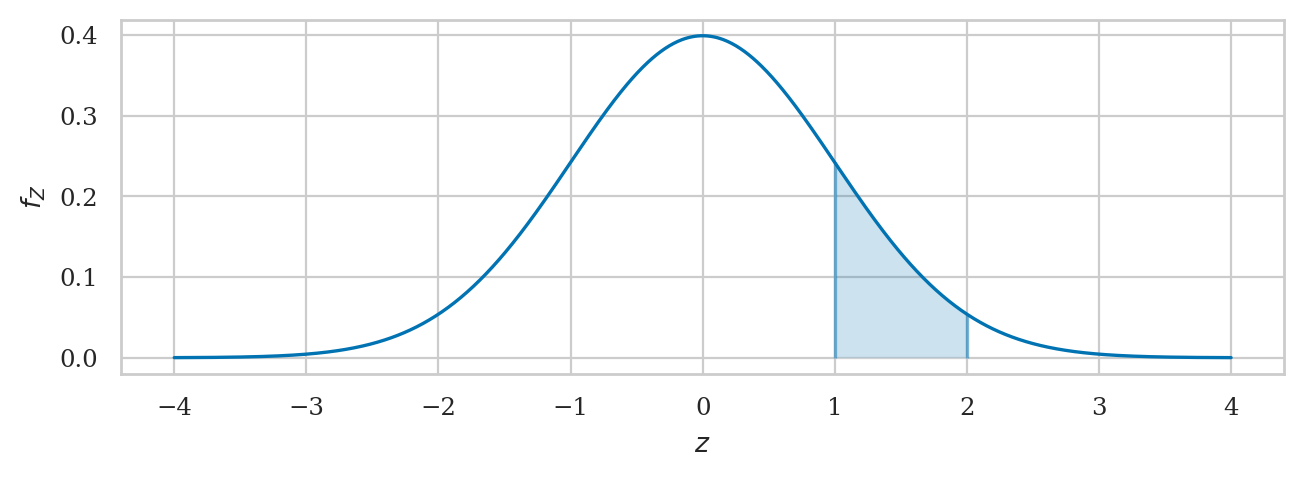
from ministats import plot_pdf

plot_pdf(rvZ, xlims=[-4,4], rv_name="Z", a=1, b=2);
Calculating the probability of an event#
The code example below shows the calculation of the probability \(\Pr\!\left( \{ 1 \leq Z \leq 2 \} \right)\), which corresponds to the integral \(\int_{z=1}^{z=2} f_Z(z) dz\).
We use the quad function to integrate rvZ.pdf between \(z=1\) and \(z=2\).
from scipy.integrate import quad
quad(rvZ.pdf, a=1, b=2)[0]
0.13590512198327787
The total area under the graph of \(f_Z\) is equal to \(1\).
To verify this claim, we would need to compute \(\int_{u=-\infty}^{u=\infty} f_Z(z)\,dz\), but the values of \(f_Z\) drop off to zero very quickly outside the central region, so it is sufficient to compute the integral \(\int_{u=-10}^{u=10} f_Z(z)\,dz\), which extends 10 standard deviations to the left and 10 standard deviaitons to the right.
quad(rvZ.pdf, a=-10, b=10)[0]
1.0000000000000002
Cumulative distribution functions#
Definitions:
\(F_X\): the cumulative distribution function (CDF) tells us the probability of an outcome less than or equal to a given value: \(F_X(b) = Pr(\{ X \leq b \})\).
\(F_X^{-1}\): the inverse cumulative distribution function computes contains the information about the quantiles of the probability distribution. The value \(F_X^{-1}(q)=x_q\) tells how far you need to go in the sample space so that the event \(\{ X \leq x_q \}\) contains a proportion \(q\) of the total probability: \(\Pr(\{ X \leq x_q \})=q\).
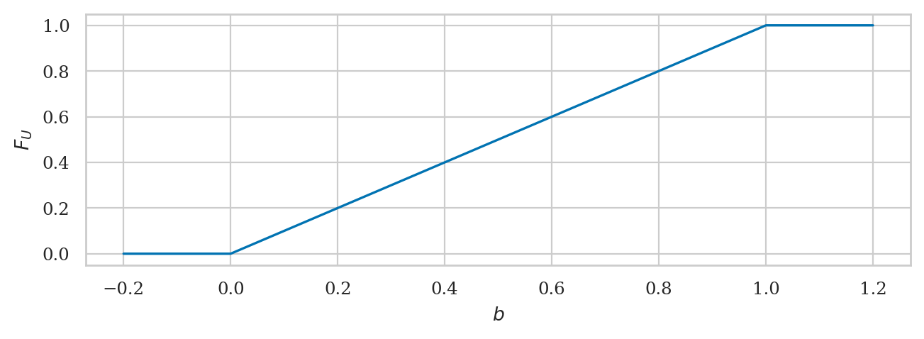
Example 1 (continued): uniform random variable#
bs = np.linspace(-0.2, 1.2, 1000)
FUs = rvU.cdf(bs)
ax = sns.lineplot(x=bs, y=FUs)
ax.set_xlabel("$b$")
ax.set_ylabel("$F_U$");
from ministats import plot_cdf
plot_cdf(rvU, xlims=[-0.2,1.2], rv_name="U");
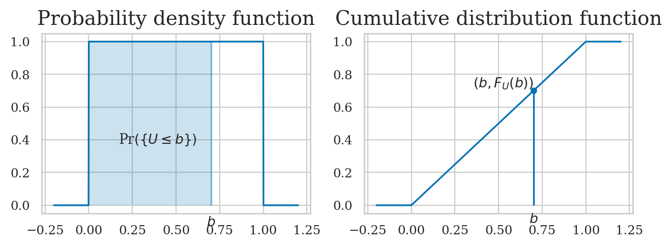
from ministats import plot_pdf_and_cdf
plot_pdf_and_cdf(rvU, b=0.7, xlims=[-0.2,1.2], rv_name="U");
rvU.cdf(0.5) - rvU.cdf(0.2)
0.3
quad(rvU.pdf, a=0.2, b=0.5)[0]
0.3
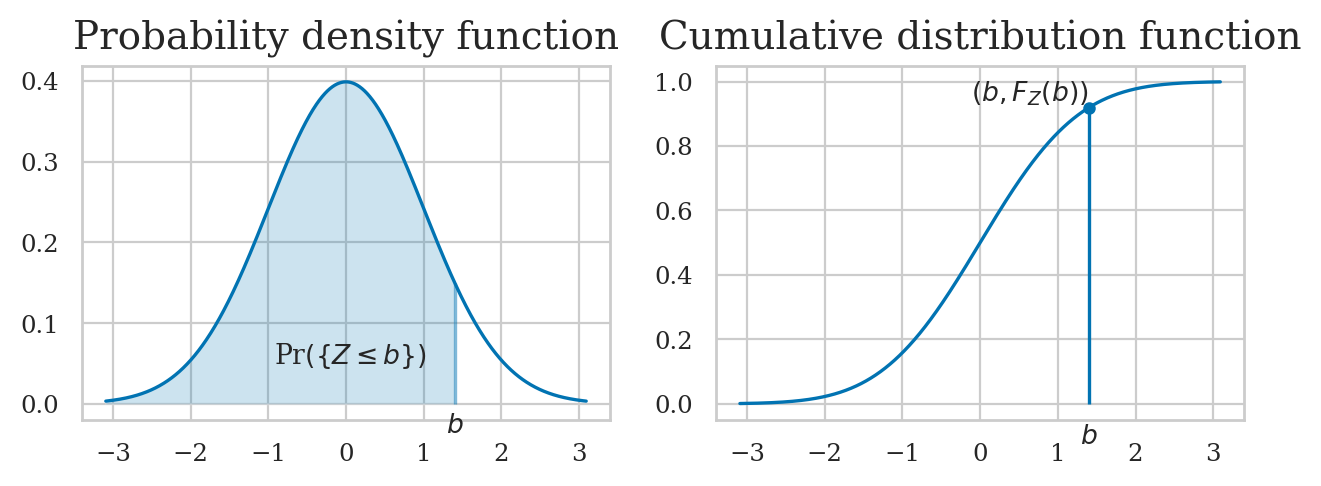
Example 2 (continued): normal random variable#
plot_pdf_and_cdf(rvZ, b=1.4, rv_name="Z");
rvZ.cdf(2) - rvZ.cdf(1)
0.13590512198327787
quad(rvZ.pdf, a=1, b=2)[0]
0.13590512198327787
Inverse of the cumulative distribution function#
rvZ.ppf(0.95)
1.6448536269514722
rvZ.cdf(1.6448536269514722)
0.95
[rvZ.ppf(0.05), rvZ.ppf(0.95)]
[-1.6448536269514729, 1.6448536269514722]
Calculating expectations#
We denote \(\mathbb{E}_X[w]\) the expected value of the function \(w(X)\) computes the average value of \(w(X)\) computed for all the possible values of the random variable \(X\).
Example 1: mean and variance of the uniform distribution#
Mean#
rvU.mean()
0.5
# # ALT. manual integration
# quad(lambda u: u*rvU.pdf(u), a=0, b=1)[0]
So the mean is \(\mu_U = \frac{1}{2} = 0.5\).
Variance#
The formula for the variance is
rvU.var()
0.08333333333333333
# # ALT. manual integration
# quad(lambda u: (u-0.5)**2*rvU.pdf(u), a=0, b=1)[0]
So the variance of \(U\) is \(\sigma_U^2 = 0.08\overline{3} = \frac{1}{12}\).
We can compute the standard deviation \(\sigma_U\) (the square root of the variance)
by calling the method rvu.std.
rvU.std()
0.28867513459481287
Example 2: mean and variance of a normal distribution#
The mean of \(Z\) is
rvZ.mean()
0.0
The variance of \(Z\) is
rvZ.var()
1.0
rvZ.std()
1.0
# ALT. manual integration
# quad(lambda z: (z-0)**2*rvZ.pdf(z), a=-10, b=10)[0]
Skewness and kurtosis#
rvZ.stats(moments="s")
0.0
rvZ.stats(moments="k")
0.0
Kombucha volume example#
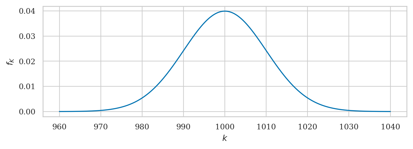
A random variable \(K\) with a normal distribution \(\mathcal{N}(\mu_K,\sigma_K)\) is described by the probability density function:
The mean \(\mu_K\) (the Greek letter mu) and the standard deviation \(\sigma_K\) (the Greek letter sigma) are called the parameters of the distribution.
The math notation \(\mathcal{N}(\mu, \sigma)\) is used to describe the whole family of normal probability distributions, and \(K \sim \mathcal{N}(\mu_K=1000, \sigma_K=10)\) is a particular instance of the distribution with mean \(\mu_K = 1000\) and standard deviation \(\sigma_K = 10\).
Create a normal random variable with mean 1000 and standard deviation 10.
from scipy.stats import norm

muK = 1000
sigmaK = 10
rvK = norm(muK, sigmaK)
# type(rvK)
# MAYBE: rvK.pdf = def fK(k) ... show Python function
Plotting the probability density function#
from ministats import plot_pdf

plot_pdf(rvK, xlims=[960,1040], rv_name="K");
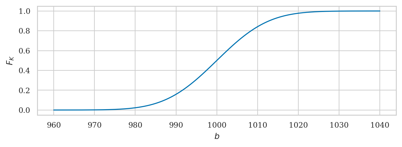
The cumulative distribution is the integral of the probability density function:
from ministats import plot_cdf

plot_cdf(rvK, xlims=[960,1040], rv_name="K");
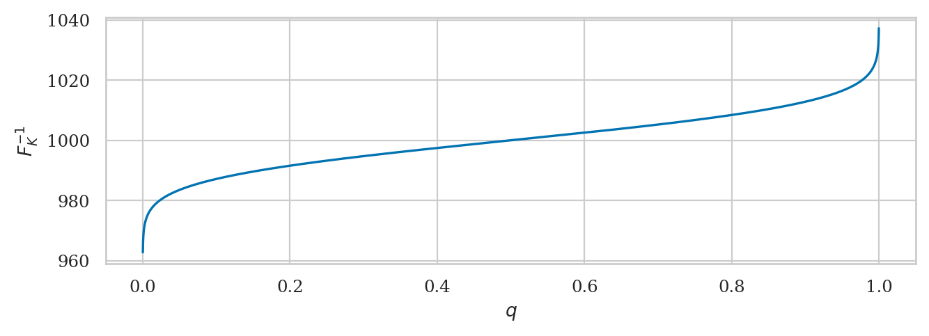
The inverse of the cumulative distribution function \(F_K^{-1}\)
is available as method rvK.ppf.
qs = np.linspace(0, 1, 10000)
invFqs = rvK.ppf(qs)
ax = sns.lineplot(x=qs, y=invFqs)
ax.set_xlabel("$q$")
ax.set_ylabel("$F_K^{-1}$");
Properties of the distribution#
rvK.mean()
1000.0
rvK.var()
100.0
rvK.std()
10.0
rvK.median()
1000.0
rvK.support()
(-inf, inf)
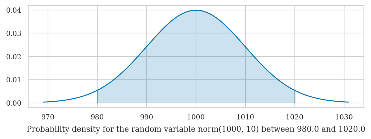
Computing probabilities#
Suppose you want to compute the probability of the outcome \(\{ 980 \leq K \leq 1020 \}\) for the random variable \(K\).
Option A: Obtain \(\textrm{Pr}(\{980 \leq N \leq 1020\})\) by calculating the integral of \(f_K\) between 980 and 1020.
quad(rvK.pdf, 980, 1020)[0]
0.9544997361036411
Option B: Obtain \(\textrm{Pr}(\{980 \leq N \leq 1020\})\) by calculating the difference in the CDF \(F_K\), \(\textrm{Pr}(\{980 \leq K \leq 1020\}) = F_K(1020) - F_K(980)\).
rvK.cdf(1020) - rvK.cdf(980)
0.9544997361036416
Computing quantiles#
Suppose we want to find the interval \((-\infty, k_q]\) that contains proportion \(q\) of the total probability. We can fing \(k_q\) by calling the inverse CDF funciton \(F_K^{-1} = \texttt{rvK.ppf}\).
First quartile#
The first quartile (\(q=0.25\) quantile) is located at \(F_K^{-1}(0.25)\):
rvK.ppf(0.25)
993.2551024980392
We can verify that \(\Pr(\{K \leq 993.255\}) = 0.25\) by calling rvK.cdf with that value.
rvK.cdf(993.2551024980392)
0.24999999999999895
Second quartile = the median#
rvK.ppf(0.5)
1000.0
Third quartile#
rvK.ppf(0.75)
1006.7448975019608
Left tail#
rvK.ppf(0.05)
983.5514637304852
Right tail#
rvK.ppf(0.95)
1016.4485362695148
Computing confidence intervals#
To compute a 90% confidence interval for the random variable \(K\),
we can call the rvK.ppf() twice.
[rvK.ppf(0.05), rvK.ppf(0.95)]
[983.5514637304852, 1016.4485362695148]
Generating random observations#
Let’s say you want to generate \(n=100\) observations from the random variable \(K\).
You can do this by calling the method rvK.rvs(100).
np.random.seed(46)

ksample = rvK.rvs(100)
ksample[0:3]
array([1005.8487584 , 1012.3119574 , 1008.21900264])
Sample mean#
np.mean(ksample)
999.3321800993151
Sample standard deviation#
np.std(ksample, ddof=1)
9.234629119029867
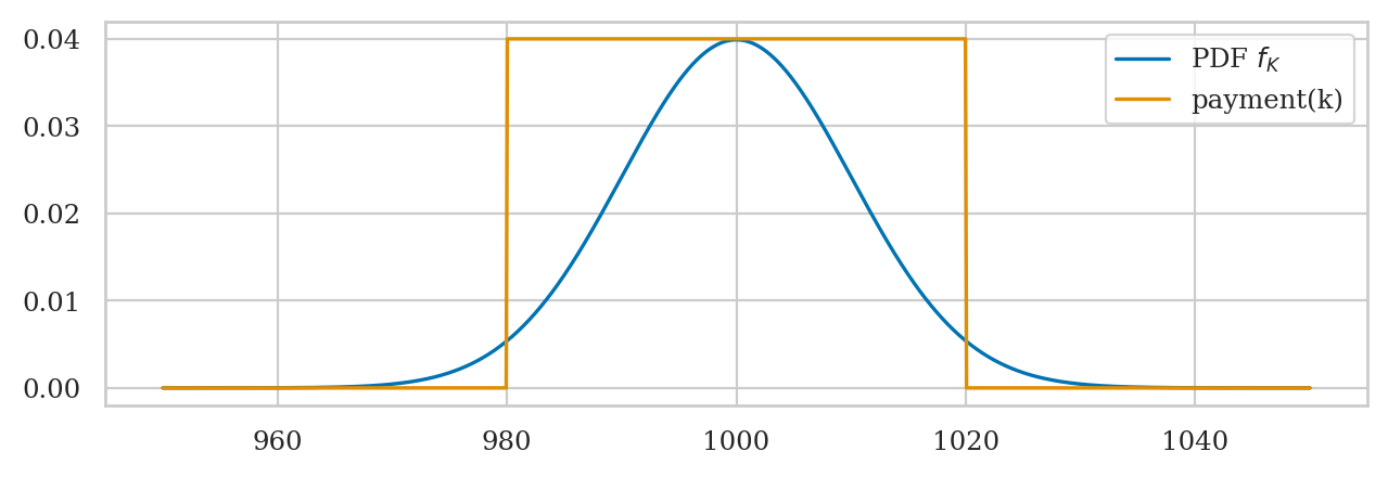
Computing expectations#
Suppose the distributor accepts only bottles contain between 980 ml and 1020 ml, and you’ll receive a receive payment of \(\$2\) for each bottle. Bottles outside that range get rejected and you don’t get paid for them.
def payment(k):
    if 980 <= k and k <= 1020:
        return 2
    else:
        return 0
# get paid if in spec
payment(1005)
2
# don't get paid if out of spec
payment(1025)
0
# expected value of payment
rvK.expect(payment, lb=-np.inf, ub=np.inf)
1.9089994604952036
Visually speaking, only the middle part of the probability distribution “counts” towards the payment. The subset that contributes to the expectation can be visualized as the values inside the rectangular region shown below.
ks = np.linspace(950, 1050, 1000)
payments = [payment(k)/50 for k in ks]

sns.lineplot(x=ks, y=rvK.pdf(ks), label="PDF $f_K$")
sns.lineplot(x=ks, y=payments, label="payment(k)");
Discussion#
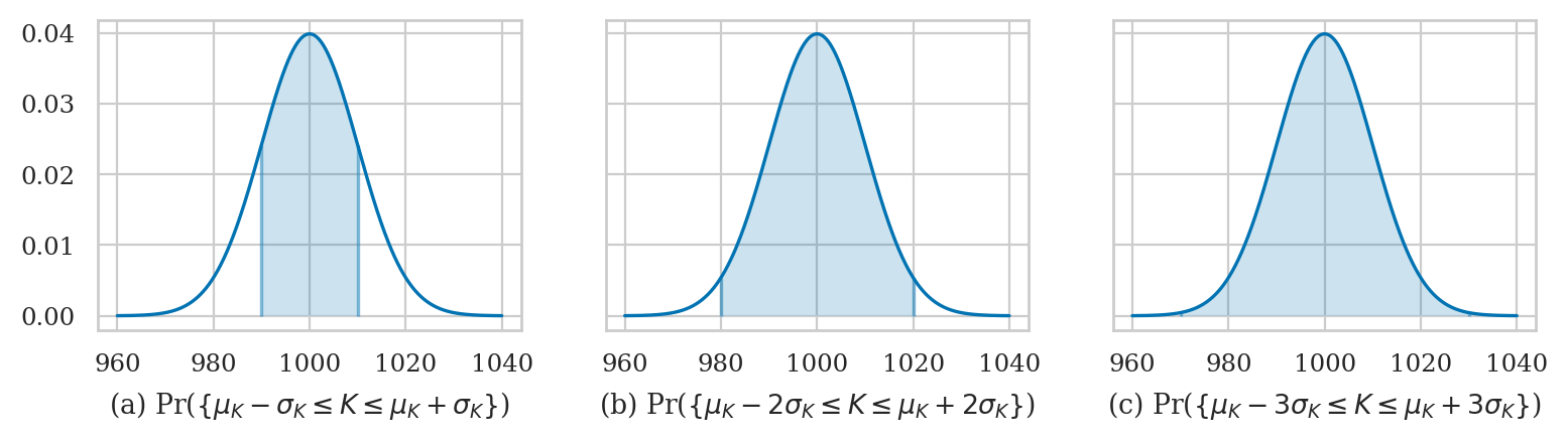
Bulk of the normal distribution#
How much of the total probability lies within \(n\) standard deviations of the mean?
from scipy.stats import norm
rvK = norm(1000, 10)
from scipy.integrate import quad

muK = rvK.mean()    # mean of the random variable rvK
sigmaK = rvK.std()  # standard deviation of rvK

for n in [2, 3]:
    I_n = [muK - n*sigmaK, muK + n*sigmaK]
    p_n = quad(rvK.pdf, I_n[0], I_n[1])[0]
    print(f"p_{n} = Pr( K in {I_n} ) = {p_n:.3f}")
p_2 = Pr( K in [980.0, 1020.0] ) = 0.954
p_3 = Pr( K in [970.0, 1030.0] ) = 0.997
The code below highlights the interval \(I_n\) and computes the probability \(p_n\).
Change the value of the variable n to get different plots.
from ministats.book.figures import bulk_of_pdf_panel

bulk_of_pdf_panel(rvK, rv_name="K", xlims=[960, 1040]);
from ministats import calc_prob_and_plot

n = 2  # number of standard deviations around the mean

# values of x in the interval 𝜇 ± n𝜎 = [𝜇-n𝜎, 𝜇+n𝜎]
I_n = [muK - n*sigmaK, muK + n*sigmaK]
p_n, _ = calc_prob_and_plot(rvK, I_n[0], I_n[1])
p_n
0.9544997361036411
Try changing the value of the variable n to 1 or 3 in the above code cell.
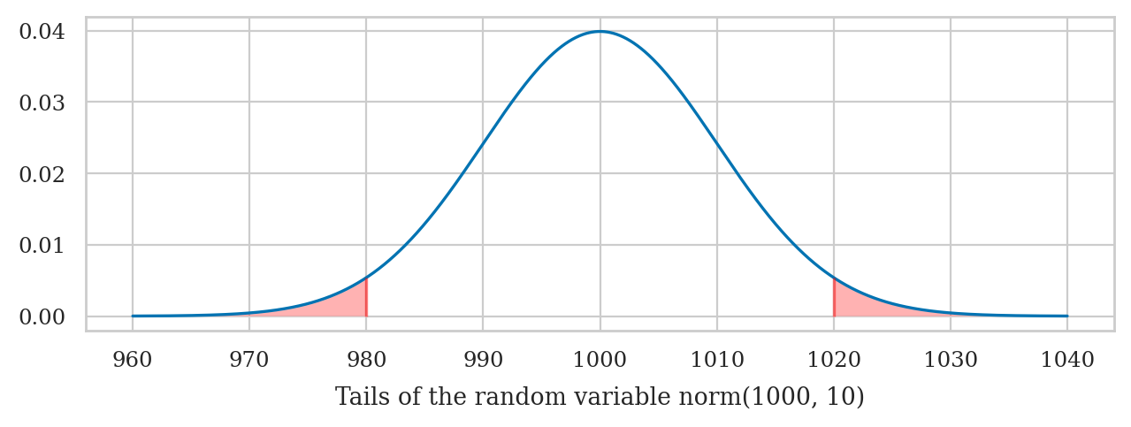
Tails of the normal distribution#
We’re often interested in tail ends of the distribution, which contain the unlikely events.
muK = rvK.mean()    # mean of the random variable rvK
sigmaK = rvK.std()  # standard deviation of rvK

for n in [2, 3]:
    # compute the probability in the left tail (-∞,𝜇-n𝜎]
    x_l = muK - n*sigmaK
    p_l = quad(rvK.pdf, -np.inf, x_l)[0]
    # compute the probability in the right tail [𝜇+n𝜎,∞)
    x_r = muK + n*sigmaK
    p_r = quad(rvK.pdf, x_r, np.inf)[0]
    # add together to get total probability in the tails
    p_tails = p_l + p_r
    print(f"Pr({{K<{x_l} or K>{x_r}}}) = {p_tails:.4f}")
Pr({K<980.0 or K>1020.0}) = 0.0455
Pr({K<970.0 or K>1030.0}) = 0.0027
The code below highlights the tails of the distribution.
from ministats import calc_prob_and_plot_tails

muK = rvK.mean()    # mean of the random variable rvK
sigmaK = rvK.std()  # standard deviation of rvK

n = 2  # number of standard deviations around the mean

# the distribution's left tail (-∞,𝜇-k𝜎]
x_l = muK - n*sigmaK

# the distribution's right tail [𝜇+k𝜎,∞)
x_r = muK + n*sigmaK

p_tails, _ = calc_prob_and_plot_tails(rvK, x_l, x_r, xlims=[960, 1040])

print(f"Pr( {{K<{x_l}}} ∪ {{K>{x_r}}} ) = {p_tails:.4f}")
Pr( {K<980.0} ∪ {K>1020.0} ) = 0.0455
Try changing the value of the variable n in the above code cell.
from ministats.book.figures import tails_of_pdf_panel

tails_of_pdf_panel(rvK, rv_name="K", xlims=[960,1040]);
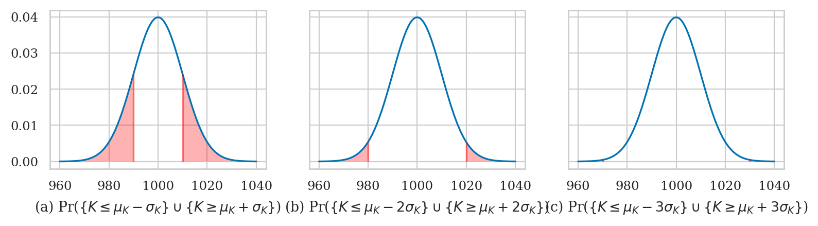
The above calculations leads us to an important rule of thumb: the values of the 5% tail of the distribution are approximately \(n=2\) standard deviations away from the mean (more precisely \(n=1.96\) to get exactly 5%). We’ll use this facts later in Chapter 3 to define events that are less than 5% likely to occur by chance.