Section 5.3 — Bayesian linear models#
This notebook contains the code examples from Section 5.3 Bayesian linear models from the No Bullshit Guide to Statistics.
See also examples in:
Bambi demos: 01_multiple_linear_regression.ipynb and 02_logistic_regression.ipynb
Notebook setup#
# Ensure required Python modules are installed
%pip install --quiet numpy scipy seaborn statsmodels bambi==0.15.0 pymc==5.23.0 ministats
[notice] A new release of pip is available: 26.1.1 -> 26.1.2
[notice] To update, run: pip install --upgrade pip
Note: you may need to restart the kernel to use updated packages.
# Load Python modules
import numpy as np
import pandas as pd
import seaborn as sns
import matplotlib.pyplot as plt
# Figures setup
plt.clf()  # needed otherwise `sns.set_theme` doesn't work
sns.set_theme(
    context="paper",
    style="whitegrid",
    palette="colorblind",
    rc={"font.family": "serif",
        "font.serif": ["Palatino", "DejaVu Serif", "serif"],
        "figure.figsize": (9,5)},
)
%config InlineBackend.figure_format = "retina"
<Figure size 640x480 with 0 Axes>
# Simple float __repr__
if int(np.__version__.split(".")[0]) >= 2:
    np.set_printoptions(legacy='1.25')

# Set random seed for repeatability
np.random.seed(42)
# Download datasets/ directory if necessary
from ministats import ensure_datasets
ensure_datasets()
datasets/ directory already exists.
# silence statsmodels kurtosistest warning when using n < 20
import warnings
warnings.filterwarnings("ignore", category=UserWarning)
warnings.filterwarnings("ignore", category=FutureWarning)
# silence ERROR messages when showing model graphs
# cf. https://github.com/pymc-devs/pymc/issues/7901
import logging
logging.getLogger("pytensor.graph.rewriting.basic").setLevel(logging.CRITICAL)
Bayesian model#
TODO: formula
TODO: graphical model diagram
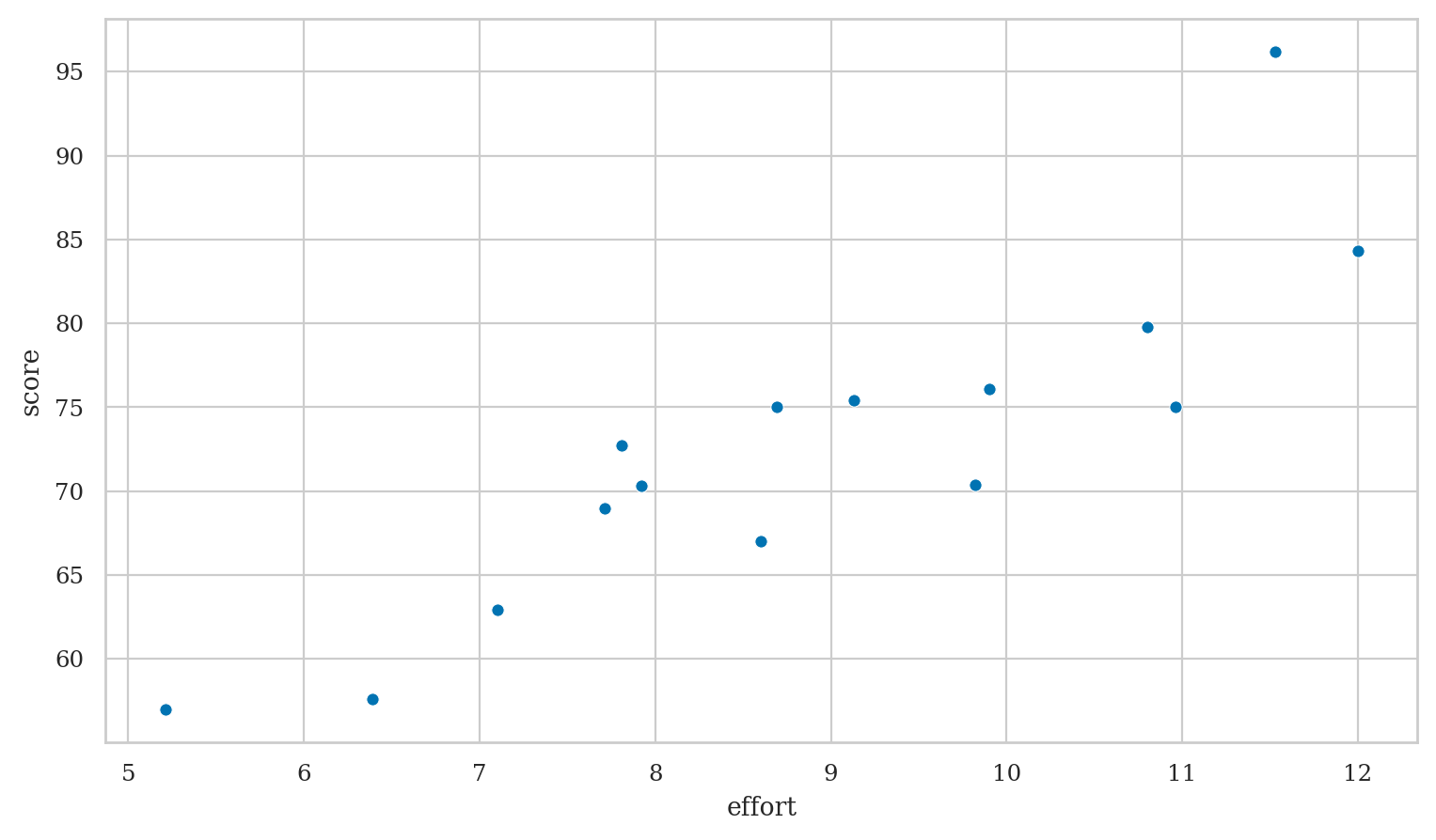
Example 1: students score as a function of effort#
Students dataset#
students = pd.read_csv("datasets/students.csv")
students.shape
(15, 5)
students.head(3)
| student_ID | background | curriculum | effort | score | |
|---|---|---|---|---|---|
| 0 | 1 | arts | debate | 10.96 | 75.0 |
| 1 | 2 | science | lecture | 8.69 | 75.0 |
| 2 | 3 | arts | debate | 8.60 | 67.0 |
students[["effort","score"]].describe().T
| count | mean | std | min | 25% | 50% | 75% | max | |
|---|---|---|---|---|---|---|---|---|
| effort | 15.0 | 8.904667 | 1.948156 | 5.21 | 7.76 | 8.69 | 10.35 | 12.0 |
| score | 15.0 | 72.580000 | 9.979279 | 57.00 | 68.00 | 72.70 | 75.75 | 96.2 |
sns.scatterplot(x="effort", y="score", data=students);
Bayesian model#
TODO: add formulas
Bambi model#
import bambi as bmb

priors1 = {
    "Intercept": bmb.Prior("Normal", mu=70, sigma=20),
    "effort": bmb.Prior("Normal", mu=0, sigma=10),
    "sigma": bmb.Prior("HalfStudentT", nu=4, sigma=10),
}

mod1 = bmb.Model("score ~ 1 + effort",
                 family="gaussian",
                 link="identity",
                 priors=priors1,
                 data=students)
Inspecting the Bambi model#
mod1
       Formula: score ~ 1 + effort
        Family: gaussian
          Link: mu = identity
  Observations: 15
        Priors:
    target = mu
        Common-level effects
            Intercept ~ Normal(mu: 70.0, sigma: 20.0)
            effort ~ Normal(mu: 0.0, sigma: 10.0)

        Auxiliary parameters
            sigma ~ HalfStudentT(nu: 4.0, sigma: 10.0)
mod1.build()
mod1.graph()

Prior predictive checks#
# TODO
Model fitting and analysis#
idata1 = mod1.fit(random_seed=42)
Initializing NUTS using jitter+adapt_diag...
Multiprocess sampling (2 chains in 2 jobs)
NUTS: [sigma, Intercept, effort]
Sampling 2 chains for 1_000 tune and 1_000 draw iterations (2_000 + 2_000 draws total) took 1 seconds.
We recommend running at least 4 chains for robust computation of convergence diagnostics
import arviz as az
az.summary(idata1, kind="stats")
| mean | sd | hdi_3% | hdi_97% | |
|---|---|---|---|---|
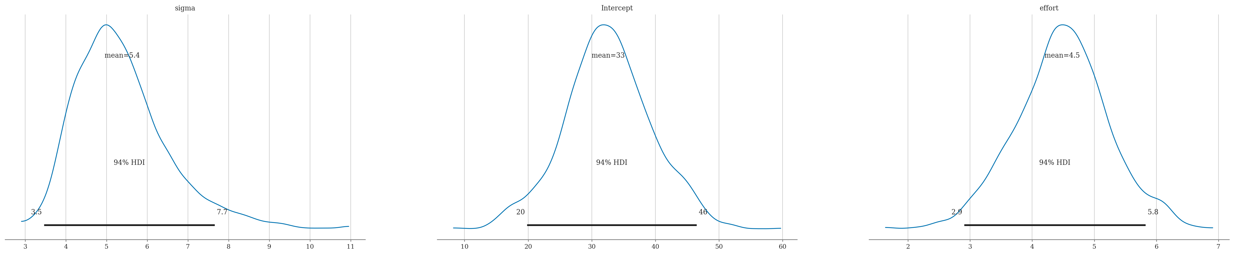
| sigma | 5.389 | 1.171 | 3.463 | 7.662 |
| Intercept | 32.573 | 6.900 | 19.826 | 46.465 |
| effort | 4.485 | 0.750 | 2.907 | 5.824 |
az.plot_posterior(idata1);
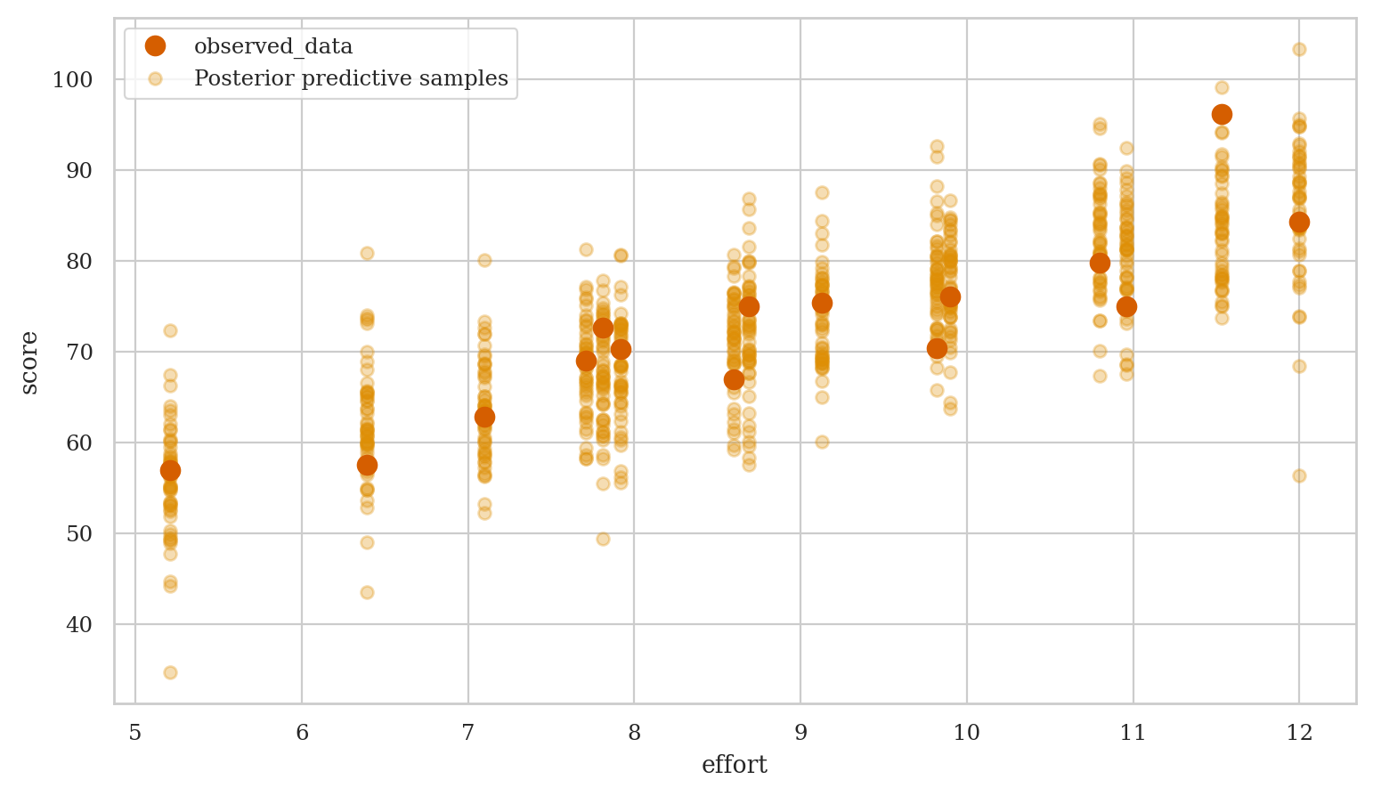
Model predictions#
Generate samples form the posterior predictive distribution,
then use the ArviZ function plot_lm to generate a complete visualization.
preds1 = mod1.predict(idata=idata1, data=students,
                      kind="response", inplace=False)
efforts = students["effort"]
az.plot_lm(y="score", idata=preds1, x=efforts,
           y_model="mu", y_hat="score",
           kind_pp="samples", kind_model="lines");
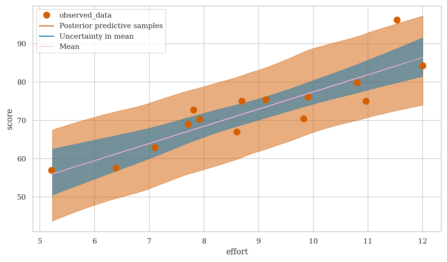
az.plot_lm(y="score", idata=preds1, x=efforts,
           y_model="mu", y_hat="score",
           kind_pp="hdi", kind_model="hdi");
Comparing to frequentist results#
For your convenience,
I’ll reproduce the statsmodels analysis from Section 4.1.
# compare with statsmodels results
import statsmodels.formula.api as smf
lm1 = smf.ols("score ~ 1 + effort", data=students).fit()
lm1.summary().tables[1]
| coef | std err | t | P>|t| | [0.025 | 0.975] | |
|---|---|---|---|---|---|---|
| Intercept | 32.4658 | 6.155 | 5.275 | 0.000 | 19.169 | 45.763 |
| effort | 4.5049 | 0.676 | 6.661 | 0.000 | 3.044 | 5.966 |
np.sqrt(lm1.scale)
4.929598282660258
lm1.conf_int(alpha=0.06) # to match 94% coverage of the Bayesian HDIs
| 0 | 1 | |
|---|---|---|
| Intercept | 19.786169 | 45.145449 |
| effort | 3.111697 | 5.898004 |
Conclusions#
We see effort tends to increase student scores. The results we obtain from the Bayesian analysis are largely consistent with the frequentist results from Section 4.1, however Bayesian models allow for simpler interpretation.
Example 2: doctors sleep scores#
Doctors dataset#
doctors = pd.read_csv("datasets/doctors.csv")
doctors.shape
(156, 9)
doctors.head(3)
| permit | loc | work | hours | caf | alc | weed | exrc | score | |
|---|---|---|---|---|---|---|---|---|---|
| 0 | 93273 | rur | hos | 21 | 2 | 0 | 5.0 | 0.0 | 63 |
| 1 | 90852 | urb | cli | 74 | 26 | 20 | 0.0 | 4.5 | 16 |
| 2 | 92744 | urb | hos | 63 | 25 | 1 | 0.0 | 7.0 | 58 |
doctors[["alc","weed","exrc","score"]].describe().T
| count | mean | std | min | 25% | 50% | 75% | max | |
|---|---|---|---|---|---|---|---|---|
| alc | 156.0 | 11.839744 | 9.428506 | 0.0 | 3.750 | 11.0 | 19.0 | 44.0 |
| weed | 156.0 | 0.628205 | 1.391068 | 0.0 | 0.000 | 0.0 | 0.5 | 10.5 |
| exrc | 156.0 | 5.387821 | 4.796361 | 0.0 | 0.875 | 4.5 | 8.0 | 19.0 |
| score | 156.0 | 48.025641 | 20.446294 | 4.0 | 33.000 | 49.5 | 62.0 | 97.0 |
Bayesian model#
TODO: add formulas
Bambi model#
priors2 = {
    "Intercept": bmb.Prior("Normal", mu=50, sigma=40),
    # we'll set the priors for the slopes below
    "sigma": bmb.Prior("HalfStudentT", nu=4, sigma=20),
}

mod2 = bmb.Model("score ~ 1 + alc + weed + exrc",
                 family="gaussian",
                 link="identity",
                 priors=priors2,
                 data=doctors)

# set the same prior for all slopes using `set_priors`
slope_prior = bmb.Prior("Normal", mu=0, sigma=10)
mod2.set_priors(common=slope_prior)

mod2
       Formula: score ~ 1 + alc + weed + exrc
        Family: gaussian
          Link: mu = identity
  Observations: 156
        Priors:
    target = mu
        Common-level effects
            Intercept ~ Normal(mu: 50.0, sigma: 40.0)
            alc ~ Normal(mu: 0.0, sigma: 10.0)
            weed ~ Normal(mu: 0.0, sigma: 10.0)
            exrc ~ Normal(mu: 0.0, sigma: 10.0)

        Auxiliary parameters
            sigma ~ HalfStudentT(nu: 4.0, sigma: 20.0)
mod2.build()
mod2.graph()

Prior predictive checks#
What kind of parameters (lines) do we get from the data model when the distribution of the parameters comes from random samples from the priors?
# TODO
Model fitting and analysis#
idata2 = mod2.fit(random_seed=42)
Initializing NUTS using jitter+adapt_diag...
Multiprocess sampling (2 chains in 2 jobs)
NUTS: [sigma, Intercept, alc, weed, exrc]
Sampling 2 chains for 1_000 tune and 1_000 draw iterations (2_000 + 2_000 draws total) took 2 seconds.
We recommend running at least 4 chains for robust computation of convergence diagnostics
az.summary(idata2, kind="stats", hdi_prob=0.95)
| mean | sd | hdi_2.5% | hdi_97.5% | |
|---|---|---|---|---|
| sigma | 8.263 | 0.503 | 7.285 | 9.250 |
| Intercept | 60.465 | 1.266 | 57.845 | 62.895 |
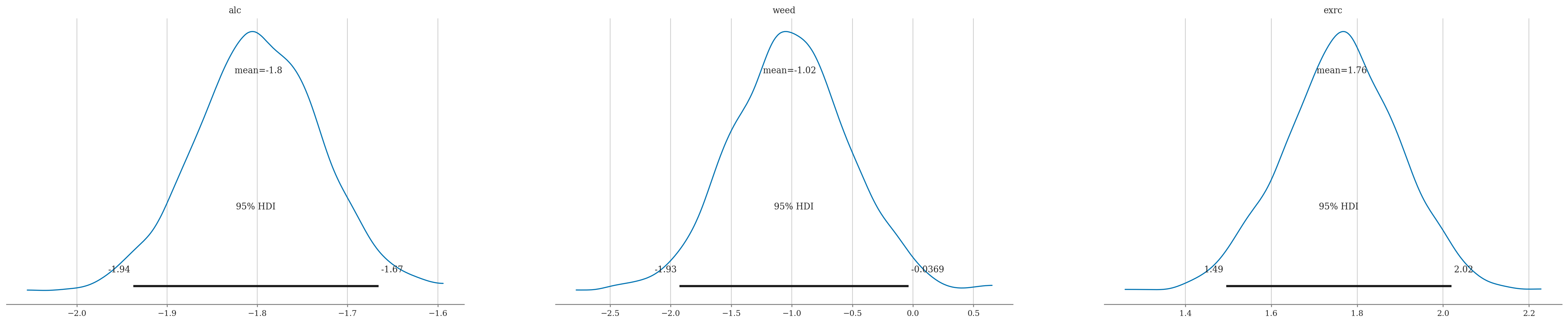
| alc | -1.799 | 0.069 | -1.938 | -1.666 |
| weed | -1.017 | 0.487 | -1.928 | -0.037 |
| exrc | 1.764 | 0.136 | 1.495 | 2.019 |
az.plot_posterior(idata2, hdi_prob=0.95, round_to=3,
                  var_names=["alc", "weed", "exrc"]);
Partial correlation scale?#
Comparing to frequentist results#
For your convenience,
I’ll reproduce the statsmodels analysis from Section 4.2.
# compare with statsmodels results
import statsmodels.formula.api as smf
formula = "score ~ 1 + alc + weed + exrc"
lm2 = smf.ols(formula, data=doctors).fit()
lm2.summary().tables[1]
| coef | std err | t | P>|t| | [0.025 | 0.975] | |
|---|---|---|---|---|---|---|
| Intercept | 60.4529 | 1.289 | 46.885 | 0.000 | 57.905 | 63.000 |
| alc | -1.8001 | 0.070 | -25.726 | 0.000 | -1.938 | -1.662 |
| weed | -1.0216 | 0.476 | -2.145 | 0.034 | -1.962 | -0.081 |
| exrc | 1.7683 | 0.138 | 12.809 | 0.000 | 1.496 | 2.041 |
np.sqrt(lm2.scale)
8.202768119825624
Conclusions#
Example 3: Bayesian logistic regression#
Interns data#
interns = pd.read_csv("datasets/interns.csv")
interns.head(3)
| work | hired | |
|---|---|---|
| 0 | 42.5 | 1 |
| 1 | 39.3 | 0 |
| 2 | 43.2 | 1 |
Bayesian logistic regression model#
Bambi model#
priors3 = {
    "Intercept": bmb.Prior("Normal", mu=0, sigma=20),
    "work": bmb.Prior("Normal", mu=2, sigma=2),
}

mod3 = bmb.Model("hired ~ 1 + work",
                 family="bernoulli",
                 link="logit",
                 priors=priors3,
                 data=interns)
mod3
       Formula: hired ~ 1 + work
        Family: bernoulli
          Link: p = logit
  Observations: 100
        Priors:
    target = p
        Common-level effects
            Intercept ~ Normal(mu: 0.0, sigma: 20.0)
            work ~ Normal(mu: 2.0, sigma: 2.0)
mod3.build()
mod3.graph()

Prior predictive checks#
# # TODO: improve prior predictive plot (currently runs too slowly)
# idatapp = mod3.prior_predictive()
# for i in range(300):
#     ps = idatapp["prior"].sel(draw=[i], chain=[0])["p"].values.flatten()
#     ws = interns["work"]
#     sps = ps[ws.sort_values().index]
#     sws = ws.sort_values().values
#     sns.lineplot(x=sws, y=sps, alpha=0.2)
Model fitting and analysis#
idata3 = mod3.fit(random_seed=42)
Modeling the probability that hired==1
Initializing NUTS using jitter+adapt_diag...
Multiprocess sampling (2 chains in 2 jobs)
NUTS: [Intercept, work]
Sampling 2 chains for 1_000 tune and 1_000 draw iterations (2_000 + 2_000 draws total) took 1 seconds.
We recommend running at least 4 chains for robust computation of convergence diagnostics
az.summary(idata3, kind="stats")
| mean | sd | hdi_3% | hdi_97% | |
|---|---|---|---|---|
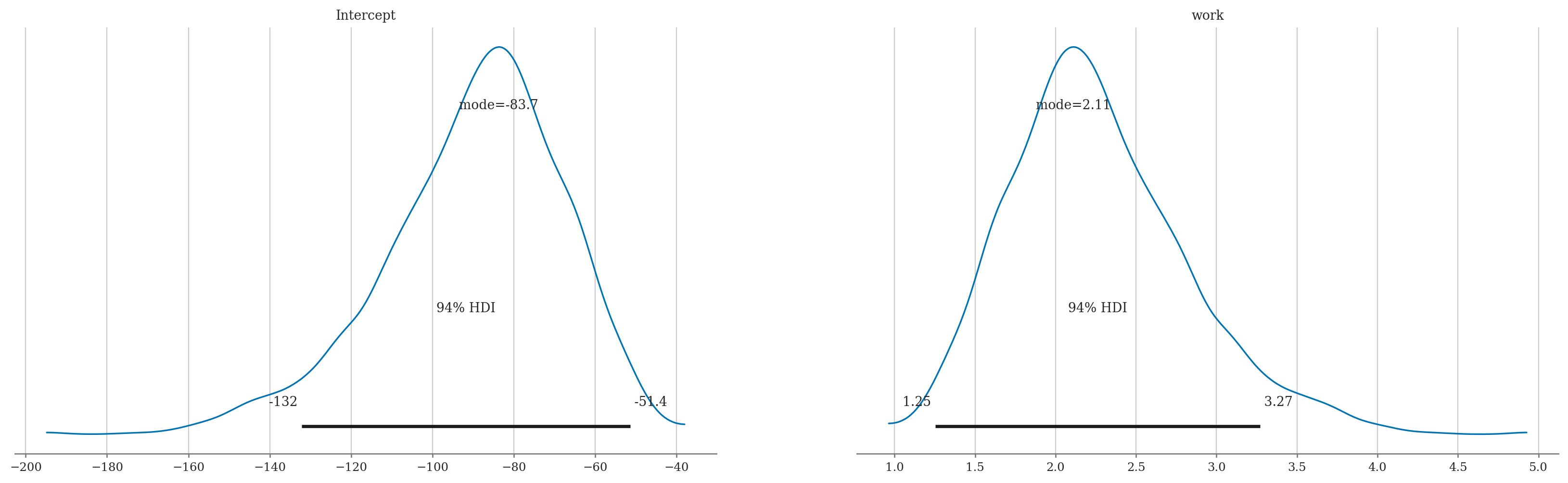
| Intercept | -89.777 | 21.906 | -132.099 | -51.382 |
| work | 2.261 | 0.552 | 1.253 | 3.271 |
az.plot_posterior(idata3, round_to=3, point_estimate="mode");
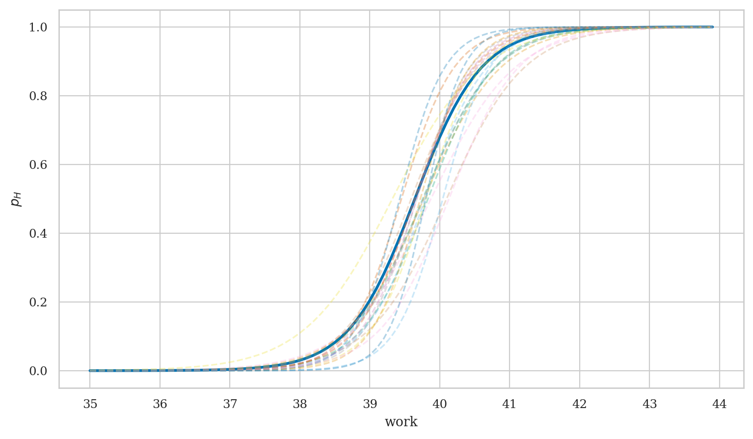
Visualize variability of the results#
from scipy.special import expit

# generate predictions
works = np.arange(35, 44, 0.1)
new_interns = pd.DataFrame({"work": works})
idata3_pred = mod3.predict(idata3, data=new_interns, inplace=False)

# plot best-fit curve based on MAP estimates
intercepts = idata3["posterior"]['Intercept'].values
wslopes = idata3["posterior"]['work'].values
B0_MAP = az.plots.plot_utils.calculate_point_estimate('mode', intercepts)
Bw_MAP = az.plots.plot_utils.calculate_point_estimate('mode', wslopes)
print("MAP estimates:", B0_MAP.round(1), Bw_MAP.round(2))
p_MAP = expit(B0_MAP + Bw_MAP*works)
ax = sns.lineplot(x=works, y=p_MAP, lw=2)

# plot 40 samples
subset = np.random.choice(1000, 10, replace=False)
post3 = idata3_pred["posterior"]
post3_subset = post3.sel(draw=subset)
for ps in az.extract(post3_subset, var_names="p").T:
    sns.lineplot(x=works, y=ps, alpha=0.3, ax=ax, ls="--")
ax.set_xlabel("work")
ax.set_ylabel("$p_H$")
ax.set_xticks(range(35,44+1));
MAP estimates: -83.7 2.11
Interpretation of the parameters#
We can interpret the results on the log-odds scale, the odds scale, or as marginal effects (slopes) at particular values of the predictor \(w\).
Parameters as changes in the log-odds#
The mode of the posterior distribution \(\widehat{B_w}_{\text{MAP}}\) corresponds to the change in log-odds per unit increase in work hours.
from ministats import mode_from_samples

post_work = idata3["posterior"]["work"].values.flatten()
mode_from_samples(post_work)
2.1091131528229434
Parameters as ratios of odds#
We can also \tt{exp}-transform this estimate to obtain the rate of increase in the odds of getting hired per additional hour of work invested.
np.exp(2.01)
7.463317347319193
Actually,
the more accurate way to summarize the odds ratio
would be to exp-transform the whole posterior distribution \(f_{B_w|\tt{interns}}\),
then find the maximum using mode_from_samples(np.exp(post_work)),
which produces the estimate \(6.81\).
Differences in probabilities#
What is the marginal effect of the predictor work
for an intern who invests 40 hours of effort?
bmb.interpret.slopes(mod3, idata3, wrt={"work":[40]}, average_by=True)
| term | estimate_type | estimate | lower_3.0% | upper_97.0% | |
|---|---|---|---|---|---|
| 0 | work | dydx | 0.474712 | 0.249691 | 0.695938 |
# ALT. manual calculation based on derivative of `expit`
# sample the parameter p from `mod3` when work=40
work40 = pd.DataFrame({"work": [40]})
preds = mod3.predict(idata3, data=work40, inplace=False)
ps40 = preds["posterior"]["p"].values.flatten()
# use the slope formula dp/dwork = p*(1-p)*beta_work
marg_effect_at_40 = ps40 * (1 - ps40) * post_work
marg_effect_at_40.mean()
0.4747284825977878
Predictions#
Let’s use the logistic regression model mod3
to predict the probability of being hired
for an intern that invests 42 hours of work per week.
work42 = pd.DataFrame({"work": [42]})
preds42 = mod3.predict(idata3, data=work42, inplace=False)
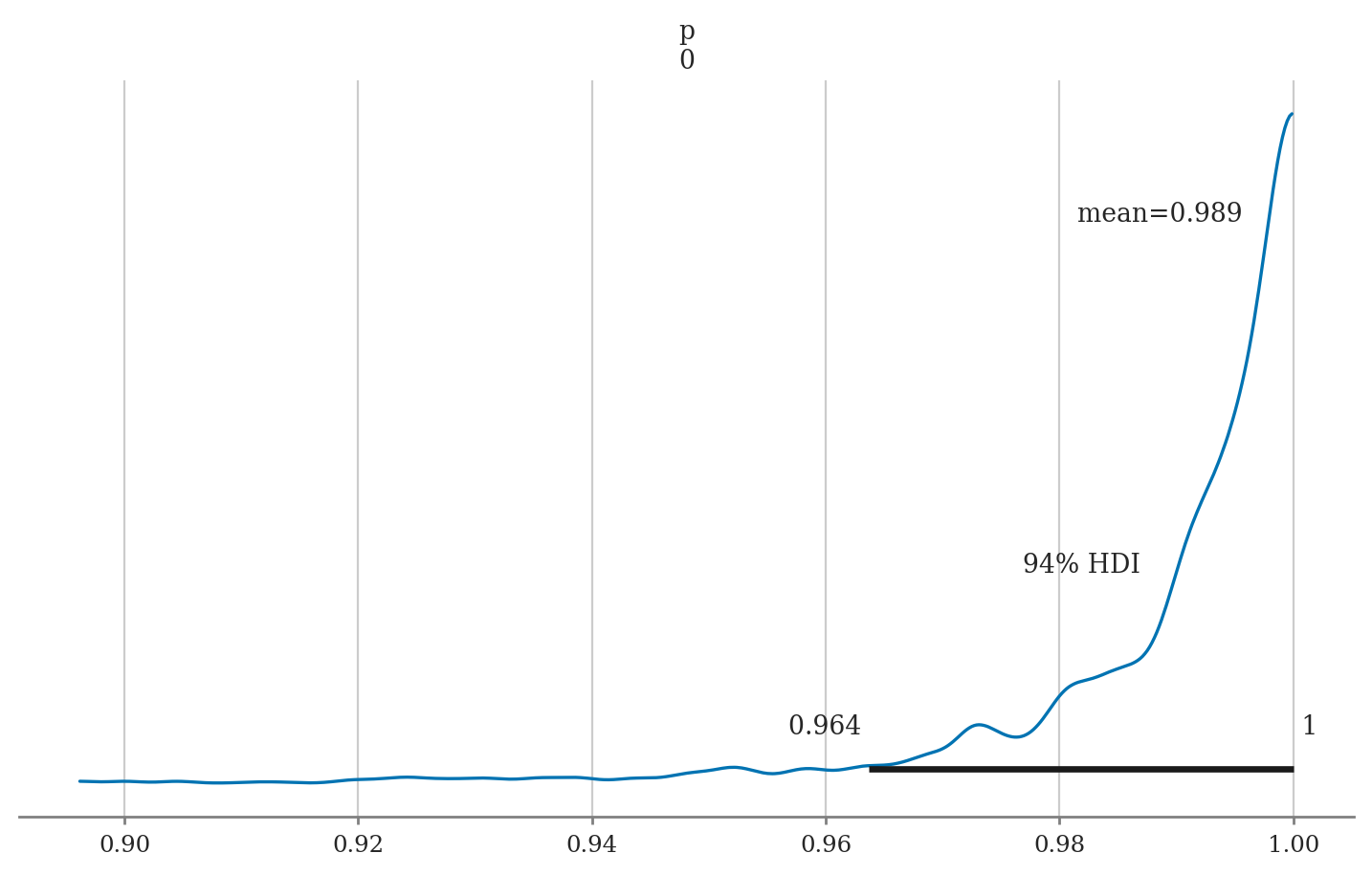
az.summary(preds42, var_names="p", kind="stats")
| mean | sd | hdi_3% | hdi_97% | |
|---|---|---|---|---|
| p[0] | 0.989 | 0.014 | 0.964 | 1.0 |
The mean model prediction is \(p(42) = 0.987 = 98.7\%\), with \(\mathbf{hdi}_{p,0.94} = [0.959, 1.0]\), which means the intern will very likely get hired.
# ALT. compute using Bambi helper function
bmb.interpret.predictions(mod3, idata3, conditional={"work":42})
| work | estimate | lower_3.0% | upper_97.0% | |
|---|---|---|---|---|
| 0 | 42.0 | 0.988604 | 0.96372 | 0.999994 |
Plot predictions#
We can visualize the predictions by plotting a histogram.
az.plot_posterior(preds42, var_names="p", round_to=3);
Comparing to frequentist results#
For your convenience,
I’ll reproduce the statsmodels analysis from Section 4.6.
import statsmodels.formula.api as smf
lr1 = smf.logit("hired ~ 1 + work", data=interns).fit()
lr1.params
Optimization terminated successfully.
         Current function value: 0.138101
         Iterations 10
Intercept   -78.693205
work          1.981458
dtype: float64
lr1.conf_int(alpha=0.06)
| 0 | 1 | |
|---|---|---|
| Intercept | -116.028234 | -41.358176 |
| work | 1.040205 | 2.922711 |
Conclusions#
We end up with similar results…
Explanations#
Robust linear regression#
We swap out the Normal distribution for Student’s \(t\)-distribution to handle outliers better very useful when data has outliers; see EXX
Links:
https://bambinos.github.io/bambi/notebooks/t_regression.html
https://www.pymc.io/examples/generalized_linear_models/GLM-robust.html
#######################################################
priors1r = {
    "Intercept": bmb.Prior("Normal", mu=70, sigma=20),
    "effort": bmb.Prior("Normal", mu=0, sigma=10),
    "sigma": bmb.Prior("HalfStudentT", nu=4, sigma=10),
    "nu": bmb.Prior("Gamma", alpha=2, beta=0.1),
}

mod1r = bmb.Model("score ~ 1 + effort",
                 family="t",
                 link="identity",
                 priors=priors1r,
                 data=students)
mod1r
       Formula: score ~ 1 + effort
        Family: t
          Link: mu = identity
  Observations: 15
        Priors:
    target = mu
        Common-level effects
            Intercept ~ Normal(mu: 70.0, sigma: 20.0)
            effort ~ Normal(mu: 0.0, sigma: 10.0)

        Auxiliary parameters
            sigma ~ HalfStudentT(nu: 4.0, sigma: 10.0)
            nu ~ Gamma(alpha: 2.0, beta: 0.1)
idata1r = mod1r.fit(random_seed=42)
Initializing NUTS using jitter+adapt_diag...
Multiprocess sampling (2 chains in 2 jobs)
NUTS: [sigma, nu, Intercept, effort]
Sampling 2 chains for 1_000 tune and 1_000 draw iterations (2_000 + 2_000 draws total) took 2 seconds.
We recommend running at least 4 chains for robust computation of convergence diagnostics
az.summary(idata1r, kind="stats")
| mean | sd | hdi_3% | hdi_97% | |
|---|---|---|---|---|
| sigma | 4.884 | 1.166 | 2.862 | 6.991 |
| nu | 19.088 | 13.259 | 1.613 | 43.700 |
| Intercept | 33.979 | 6.539 | 21.345 | 45.399 |
| effort | 4.315 | 0.737 | 2.995 | 5.734 |
The mean of the slope \(4.303\) is slightly less than the mean slope we found in mod1 (\(4.497\)),
which shows the robust model doesn’t care as much about the one outlier.
We also found a slightly smaller sigma, since we’re using the \(t\)-distribution.
Shrinkage priors#
Shrinkage priors = Prior distributions for a parameter that shrink its posterior estimate towards a particular value. Sparsity = A situation where most parameter values are zero and only a few are non-zero.
Laplace priors L1 regularization = lasso regression https://en.wikipedia.org/wiki/Lasso_(statistics)
Gaussian priors L2 regularization = ridge regression https://en.wikipedia.org/wiki/Ridge_regression
Reference priors Reference prior ppal pha, beta, sigmaq91{sigma Produces the same results as frequentist linear regression
Spike-and-slab priors Specialized for spike-and-slab prior = mix- ture of two distributions: one peaked around zero (spike) and the other a diffuse distribution (slab. The spike component identifies the zero elements whereas the slab component captures the non-zero coefficients.
Standardizing predictors#
We make choosing priors easier makes inference more efficient cf. 04_lm/cut_material/standardized_predictors.tex Robust linear regression
Discussion#
Comparison to frequentist linear models#
We can obtain similar results
Bayesian models naturally apply regularization (no need to manually add in)
Causal graphs#
Causal graphs also used with Bayesian LMs (remember Sec 4.5)
Next steps#
LMs work with categorical predators too, which is what we’ll discuss in Section 5.4
LMs can be extended hierarchical models, which is what we’ll discuss in Section 5.5
Exercises#
Exercise 1: redo some of the exercises/problems from Ch4 using Bayesian methods#
Exercise 2: redo examples of causal inference#
Exercise 3: fit model with different priors#
Exercise 4: redo logistic regression exercises from Sec 4.6#
Exercise 5: bioassay logistic regression#
Gelman et al. (2003) present an example of an acute toxicity test, commonly performed on animals to estimate the toxicity of various compounds.
In this dataset log_dose includes 4 levels of dosage, on the log scale, each administered to 5 rats during the experiment. The response variable is death, the number of positive responses to the dosage.
The number of deaths can be modeled as a binomial response, with the probability of death being a linear function of dose:
The common statistic of interest in such experiments is the LD50, the dosage at which the probability of death is 50%.
# Sample size in each group
n = 5

# Log dose in each group
log_dose = [-.86, -.3, -.05, .73]

# Outcomes
deaths = [0, 1, 3, 5]

df_bio = pd.DataFrame({"log_dose":log_dose, "deaths":deaths, "n":n})
# SOLUTION
priors_bio = {
    "Intercept": bmb.Prior("Normal", mu=0, sigma=5),
    "log_dose": bmb.Prior("Normal", mu=0, sigma=5),
}

mod_bio = bmb.Model(formula="p(deaths,n) ~ 1 + log_dose",
                    family="binomial",
                    link="logit",
                    priors=priors_bio,
                    data=df_bio)

idata_bio = mod_bio.fit()

post_bio = idata_bio["posterior"]
post_bio["LD50"] = -post_bio["Intercept"] / post_bio["log_dose"]

az.summary(idata_bio)
Initializing NUTS using jitter+adapt_diag...
Multiprocess sampling (2 chains in 2 jobs)
NUTS: [Intercept, log_dose]
Sampling 2 chains for 1_000 tune and 1_000 draw iterations (2_000 + 2_000 draws total) took 1 seconds.
We recommend running at least 4 chains for robust computation of convergence diagnostics
| mean | sd | hdi_3% | hdi_97% | mcse_mean | mcse_sd | ess_bulk | ess_tail | r_hat | |
|---|---|---|---|---|---|---|---|---|---|
| Intercept | 0.590 | 0.768 | -0.703 | 2.219 | 0.022 | 0.021 | 1256.0 | 923.0 | 1.0 |
| log_dose | 6.288 | 2.496 | 2.006 | 10.874 | 0.076 | 0.060 | 1106.0 | 1337.0 | 1.0 |
| LD50 | -0.084 | 0.131 | -0.310 | 0.170 | 0.004 | 0.005 | 1399.0 | 1103.0 | 1.0 |
Exercise 6: redo Poisson regression exercises from Sec 4.6#
Exercise 7: fit normal and robust to the dataset ??TODO?? which has outliers#
Exercise 8: PhD delays#
cf. https://www.rensvandeschoot.com/tutorials/advanced-bayesian-regression-in-jasp/
https://zenodo.org/records/3999424
https://sci-hub.se/https://www.nature.com/articles/ s43586-020-00001-2
Links#
BONUS MATERIAL#
Simple linear regression using PyMC#
(used in Chapter 4 conclusion)
# Linear regression model in PyMC
students = pd.read_csv("datasets/students.csv")

import pymc as pm
with pm.Model() as model:
    # Define the priors
    B0 = pm.Normal("B0", mu=30, sigma=20)
    Be = pm.Normal("Be", mu=0, sigma=10)
    Sigma = pm.HalfStudentT("Sigma", nu=4, sigma=10)

    # Define the data model
    M = B0 + Be * students["effort"]
    S = pm.Normal("S", mu=M, sigma=Sigma, observed=students["score"])

    # Fit the model
    idata = pm.sample()
Initializing NUTS using jitter+adapt_diag...
Multiprocess sampling (2 chains in 2 jobs)
NUTS: [B0, Be, Sigma]
Sampling 2 chains for 1_000 tune and 1_000 draw iterations (2_000 + 2_000 draws total) took 3 seconds.
There were 5 divergences after tuning. Increase `target_accept` or reparameterize.
We recommend running at least 4 chains for robust computation of convergence diagnostics
import arviz as az
az.summary(idata, kind="stats")
| mean | sd | hdi_3% | hdi_97% | |
|---|---|---|---|---|
| B0 | 32.708 | 6.286 | 20.950 | 44.752 |
| Be | 4.478 | 0.688 | 3.272 | 5.870 |
| Sigma | 5.381 | 1.152 | 3.425 | 7.442 |
# cf. with Bambi results for the same model
az.summary(idata1, kind="stats")
| mean | sd | hdi_3% | hdi_97% | |
|---|---|---|---|---|
| sigma | 5.389 | 1.171 | 3.463 | 7.662 |
| Intercept | 32.573 | 6.900 | 19.826 | 46.465 |
| effort | 4.485 | 0.750 | 2.907 | 5.824 |
Simple linear regression on synthetic data#
# Simulated data
np.random.seed(42)
x = np.random.normal(0, 1, 100)
y = 3 + 2 * x + np.random.normal(0, 1, 100)
df1 = pd.DataFrame({"x":x, "y":y})

priors1 = {
    "Intercept": bmb.Prior("Normal", mu=0, sigma=10),
    "x": bmb.Prior("Normal", mu=0, sigma=10),
    "sigma": bmb.Prior("HalfNormal", sigma=1),
}

model1 = bmb.Model("y ~ 1 + x",
                   priors=priors1,
                   data=df1)
print(model1)

idata = model1.fit(random_seed=42)
Initializing NUTS using jitter+adapt_diag...
       Formula: y ~ 1 + x
        Family: gaussian
          Link: mu = identity
  Observations: 100
        Priors:
    target = mu
        Common-level effects
            Intercept ~ Normal(mu: 0.0, sigma: 10.0)
            x ~ Normal(mu: 0.0, sigma: 10.0)

        Auxiliary parameters
            sigma ~ HalfNormal(sigma: 1.0)
Multiprocess sampling (2 chains in 2 jobs)
NUTS: [sigma, Intercept, x]
/opt/hostedtoolcache/Python/3.12.13/x64/lib/python3.12/site-packages/pymc/step_methods/hmc/quadpotential.py:316: RuntimeWarning: overflow encountered in dot
  return 0.5 * np.dot(x, v_out)
Sampling 2 chains for 1_000 tune and 1_000 draw iterations (2_000 + 2_000 draws total) took 1 seconds.
We recommend running at least 4 chains for robust computation of convergence diagnostics
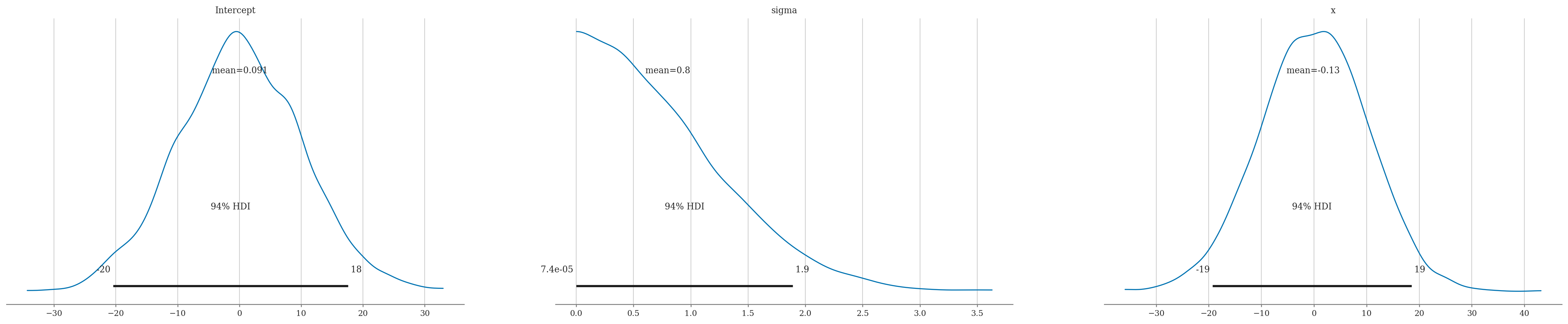
model1.plot_priors();
Sampling: [Intercept, sigma, x]
Summary using mean#
# Posterior Summary
summary = az.summary(idata, kind="stats")
summary
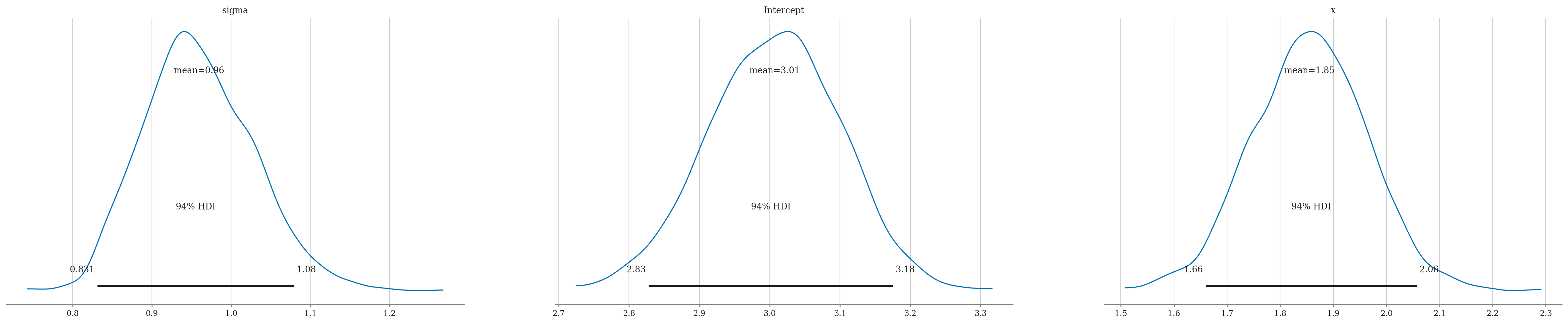
| mean | sd | hdi_3% | hdi_97% | |
|---|---|---|---|---|
| sigma | 0.960 | 0.070 | 0.831 | 1.079 |
| Intercept | 3.007 | 0.093 | 2.828 | 3.175 |
| x | 1.855 | 0.108 | 1.660 | 2.057 |
Summary using median as focus statistic#
ETI = Equal-Tailed Interval
az.summary(idata, stat_focus="median", kind="stats")
| median | mad | eti_3% | eti_97% | |
|---|---|---|---|---|
| sigma | 0.954 | 0.047 | 0.841 | 1.099 |
| Intercept | 3.008 | 0.063 | 2.829 | 3.179 |
| x | 1.855 | 0.071 | 1.657 | 2.056 |
# Plotting posterior
az.plot_posterior(idata, point_estimate="mean", round_to=3);
Investigare further
https://python.arviz.org/en/latest/api/generated/arviz.plot_lm.html
# az.plot_lm(idata)
Bonus Bayesian logistic regression example#
via file:///Users/ivan/Downloads/talks-main/pydataglobal21/index.html#15
import bambi as bmb
data = bmb.load_data("ANES")
data.head()
| vote | age | party_id | |
|---|---|---|---|
| 0 | clinton | 56 | democrat |
| 1 | trump | 65 | republican |
| 2 | clinton | 80 | democrat |
| 3 | trump | 38 | republican |
| 4 | trump | 60 | republican |
model = bmb.Model("vote[clinton] ~ 0 + party_id + party_id:age", data, family="bernoulli")
print(model)
idata = model.fit(random_seed=42)
Modeling the probability that vote==clinton
Initializing NUTS using jitter+adapt_diag...
       Formula: vote[clinton] ~ 0 + party_id + party_id:age
        Family: bernoulli
          Link: p = logit
  Observations: 421
        Priors:
    target = p
        Common-level effects
            party_id ~ Normal(mu: [0. 0. 0.], sigma: [1. 1. 1.])
            party_id:age ~ Normal(mu: [0. 0. 0.], sigma: [0.0586 0.0586 0.0586])
Multiprocess sampling (2 chains in 2 jobs)
NUTS: [party_id, party_id:age]
Sampling 2 chains for 1_000 tune and 1_000 draw iterations (2_000 + 2_000 draws total) took 5 seconds.
We recommend running at least 4 chains for robust computation of convergence diagnostics
import pandas as pd
new_subjects = pd.DataFrame({"age": [20, 60], "party_id": ["independent"] * 2})
model.predict(idata, data=new_subjects)

# TODO: try to repdouce
# https://github.com/tomicapretto/talks/blob/main/pydataglobal21/index.Rmd#L181-L193
One more example#
via http://www.medicine.mcgill.ca/epidemiology/joseph/courses/EPIB-682/bayesreg.pdf
Fit a logistic regression model of bone fractures with independent variables age and sex.
The true model had: \(\beta_0 = -25\), \(\beta_{\tt{sex}} = 0.5\), \(\beta_{\tt{age}} = 0.4\).
With so few data points and three parameters to estimate, do not expect posterior means/medians to equal the correct values exactly, but all would most likely be in the 95% intervals.
dfmed = pd.DataFrame(
    dict(sex=[1, 1, 1, 0, 1, 1, 0, 0, 0, 0, 1, 1, 1, 1, 1, 0, 1, 0, 0, 0, 1, 1, 1, 0, 0, 1, 1, 0, 1, 1, 1, 0, 0, 0, 1, 1, 0, 0, 1, 1, 0, 1, 0, 0, 0, 1, 0, 0, 0, 1, 0, 1, 0, 1, 1, 1, 0, 0, 1, 1, 1, 1, 0, 0, 0, 1, 1, 1, 0, 0, 1, 1, 1, 0, 0, 0, 1, 1, 0, 0, 0, 0, 1, 0, 0, 1, 1, 1, 0, 1, 0, 1, 1, 1, 0, 1, 1, 1, 1, 1],
         age=[69, 57, 61, 60, 69, 74, 63, 68, 64, 53, 60, 58, 79, 56, 53, 74, 56, 76, 72, 56, 66, 52, 77, 70, 69, 76, 72, 53, 69, 59, 73, 77, 55, 77, 68, 62, 56, 68, 70, 60, 65, 55, 64, 75, 60, 67, 61, 69, 75, 68, 72, 71, 54, 52, 54, 50, 75, 59, 65, 60, 60, 57, 51, 51, 63, 57, 80, 52, 65, 72, 80, 73, 76, 79, 66, 51, 76, 75, 66, 75, 78, 70, 67, 51, 70, 71, 71, 74, 74, 60, 58, 55, 61, 65, 52, 68, 75, 52, 53, 70],
         frac=[1, 1, 1, 0, 1, 1, 0, 1, 1, 0, 1, 0, 1, 1, 0, 1, 0, 1, 1, 0, 1, 0, 1, 1, 1, 1, 1, 0, 1, 0, 1, 1, 0, 1, 1, 1, 0, 1, 1, 0, 1, 0, 0, 1, 0, 1, 0, 1, 1, 1, 1, 1, 0, 0, 0, 0, 1, 1, 1, 1, 1, 0, 0, 0, 1, 0, 1, 0, 0, 1, 1, 1, 1, 1, 0, 0, 1, 1, 0, 1, 1, 1, 0, 0, 1, 1, 1, 1, 1, 1,
1, 0, 1, 1, 0, 0, 1, 0, 0, 1])
)
# df3
priorsmed = {
    "Intercept": bmb.Prior("Normal", mu=0, sigma=1e4),
    "sex": bmb.Prior("Normal", mu=0, sigma=1e4),
    "age": bmb.Prior("Normal", mu=0, sigma=1e4),
}

modmed = bmb.Model("frac ~ 1 + sex + age",
                 family="bernoulli",
                 link="logit",
                 priors=priorsmed,
                 data=dfmed)
modmed
       Formula: frac ~ 1 + sex + age
        Family: bernoulli
          Link: p = logit
  Observations: 100
        Priors:
    target = p
        Common-level effects
            Intercept ~ Normal(mu: 0.0, sigma: 10000.0)
            sex ~ Normal(mu: 0.0, sigma: 10000.0)
            age ~ Normal(mu: 0.0, sigma: 10000.0)
idatamed = modmed.fit(draws=2000, random_seed=42)
az.summary(idatamed, kind="stats")
Modeling the probability that frac==1
Initializing NUTS using jitter+adapt_diag...
Multiprocess sampling (2 chains in 2 jobs)
NUTS: [Intercept, sex, age]
Sampling 2 chains for 1_000 tune and 2_000 draw iterations (2_000 + 4_000 draws total) took 2 seconds.
We recommend running at least 4 chains for robust computation of convergence diagnostics
| mean | sd | hdi_3% | hdi_97% | |
|---|---|---|---|---|
| Intercept | -23.783 | 4.839 | -33.024 | -15.210 |
| sex | 1.526 | 0.795 | 0.012 | 2.954 |
| age | 0.375 | 0.075 | 0.239 | 0.513 |
import statsmodels.formula.api as smf
lrmed = smf.logit("frac ~ 1 + sex + age", data=dfmed).fit()
lrmed.params
Optimization terminated successfully.
         Current function value: 0.297593
         Iterations 8
Intercept   -21.850408
sex           1.361099
age           0.344670
dtype: float64