Section 3.4 — Hypothesis testing using analytical approximations#
This notebook contains the code examples from Section 3.4 Hypothesis testing using analytical approximations of the No Bullshit Guide to Statistics.
Notebook setup#
# Ensure required Python modules are installed
%pip install --quiet numpy scipy seaborn pandas ministats
Note: you may need to restart the kernel to use updated packages.
# load Python modules
import os
import numpy as np
import pandas as pd
import seaborn as sns
import matplotlib.pyplot as plt
# Figures setup
plt.clf()  # needed otherwise `sns.set_theme` doesn't work
sns.set_theme(
    context="paper",
    style="whitegrid",
    palette="colorblind",
    rc={"font.family": "serif",
        "font.serif": ["Palatino", "DejaVu Serif", "serif"],
        "figure.figsize": (5, 1.6)},
)
%config InlineBackend.figure_format = 'retina'
<Figure size 640x480 with 0 Axes>
# Simple float __repr__
if int(np.__version__.split(".")[0]) >= 2:
    np.set_printoptions(legacy='1.25')

# set random seed for repeatability
np.random.seed(42)
# Download datasets/ directory if necessary
from ministats import ensure_datasets
ensure_datasets()
datasets/ directory already exists.
\(\def\stderr#1{\mathbf{se}_{#1}}\) \(\def\stderrhat#1{\hat{\mathbf{se}}_{#1}}\) \(\newcommand{\Mean}{\textbf{Mean}}\) \(\newcommand{\Var}{\textbf{Var}}\) \(\newcommand{\Std}{\textbf{Std}}\) \(\newcommand{\Freq}{\textbf{Freq}}\) \(\newcommand{\RelFreq}{\textbf{RelFreq}}\) \(\newcommand{\DMeans}{\textbf{DMeans}}\) \(\newcommand{\Prop}{\textbf{Prop}}\) \(\newcommand{\DProps}{\textbf{DProps}}\)
(this cell contains the macro definitions like \(\stderr{\overline{\mathbf{x}}}\), \(\stderrhat{}\), \(\Mean\), …)
Definitions#
Context#
test statistic
sampling distribution of the test statistic
pivotal transformation
reference distributions
def mean(sample):
    return sum(sample) / len(sample)

def var(sample):
    xbar = mean(sample)
    sumsqdevs = sum([(xi-xbar)**2 for xi in sample])
    return sumsqdevs / (len(sample)-1)

def std(sample):
    s2 = var(sample)
    return np.sqrt(s2)
Analytical approximations#
# theoretical model for the kombucha volumes
muX0 = 1000   # population mean (expected kombucha volume)
sigmaX0 = 10  # population standard deviation
sample = [1005.19,  987.31, 1002.4,  991.96,
          1000.17, 1003.94, 1012.79]
n = len(sample)  # sample size
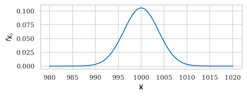
Normal approximation to the sample mean#
from scipy.stats import norm

sigmaX0 = 10  # population standard deviation
se = sigmaX0 / np.sqrt(n)
rvNXbar_0 = norm(loc=muX0, scale=se)
from ministats import plot_pdf
ax = plot_pdf(rvNXbar_0, xlims=[980, 1020])
ax.set_ylabel(r"$f_{\overline{\mathbf{X}}_0}$")
ax.set_xlabel(r"$\overline{\mathbf{x}}$");
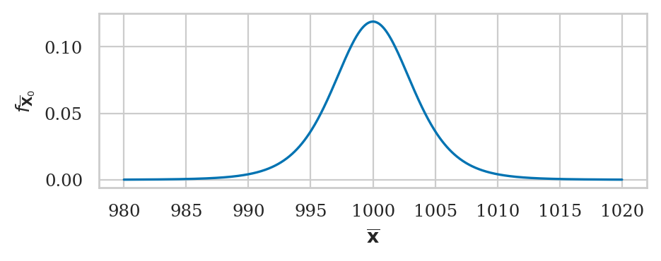
Student’s \(t\)-approximation to the sample mean#
from scipy.stats import t as tdist

muX0 = 1000      # population mean (expected kombucha volume)
sigmaX0 = 10     # population standard deviation
n = len(sample)  # sample size
sehat = std(sample) / np.sqrt(n)
rvTXbar_0 = tdist(df=n-1, loc=muX0, scale=sehat)
ax = plot_pdf(rvTXbar_0, xlims=[980, 1020])
ax.set_ylabel(r"$f_{\overline{\mathbf{X}}_0}$")
ax.set_xlabel(r"$\overline{\mathbf{x}}$");
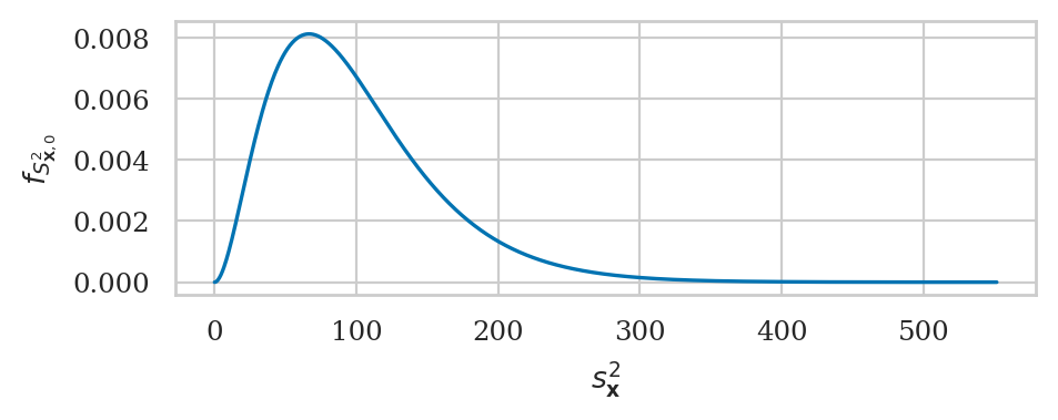
The \(\chi^2\)-approximation to the sample variance#
from scipy.stats import chi2
sigmaX0 = 10     # population standard deviation
n = len(sample)  # sample size
scale = sigmaX0**2 / (n-1)
rvQS2_0 = chi2(df=n-1, scale=scale)
ax = plot_pdf(rvQS2_0, rv_name="Q")
ax.set_ylabel(r"$f_{S^2_{\mathbf{X},0}}$")
ax.set_xlabel(r"$s^2_{\mathbf{x}}$");
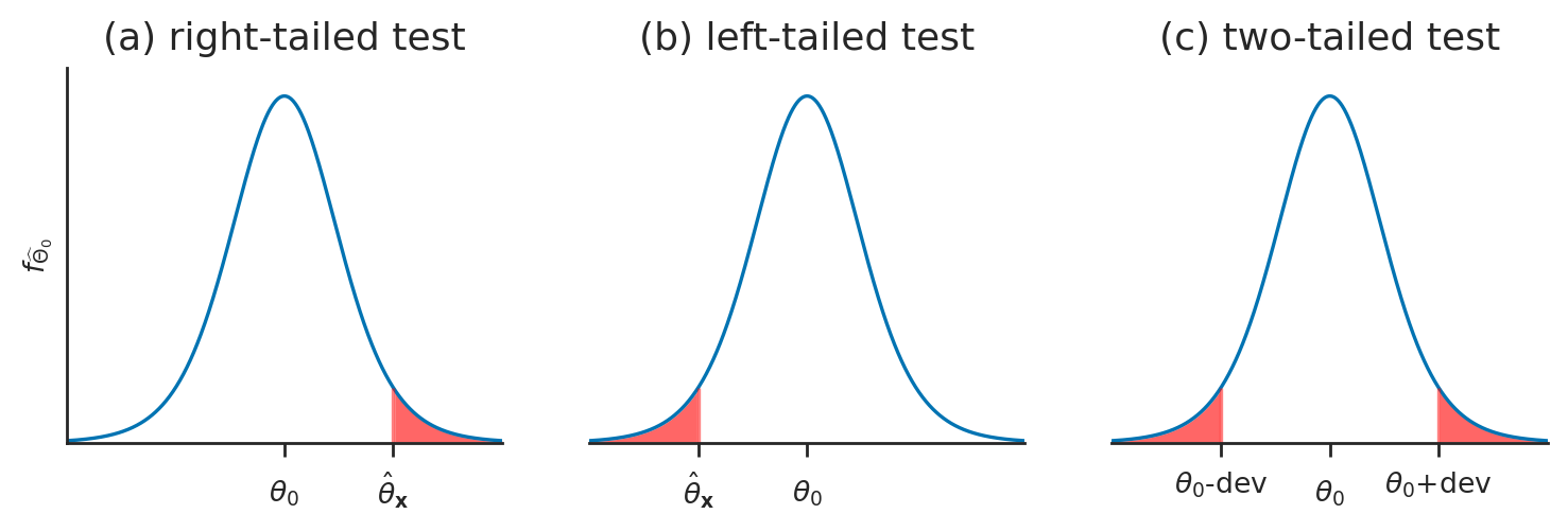
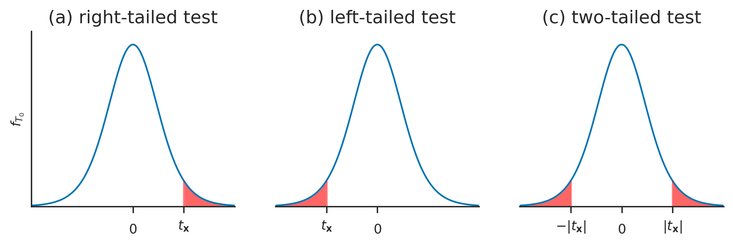
Calculating \(p\)-values#
from ministats.book.figures import plot_panel_pvalue_theta0_tails

fig = plot_panel_pvalue_theta0_tails();
Pivotal transformations#
Calculating \(p\)-values for standardized test statistics#
from ministats.book.figures import plot_panel_pvalue_t_tails

fig = plot_panel_pvalue_t_tails();
Test for the mean (known variance)#
Analytical approximation for the sample mean#
If the theoretical distribution under the null is normally distributed \(X_0 \sim \mathcal{N}(\mu_{X_0}, \sigma_{X_0})\), then the central limit theorem tells us the sampling distribution of the mean is described by the formula
Kombucha bottling process#
We’ll use the kombucha scenario for all the examples in this section. Recall, the probability distirbution of the kombucha volume is described by the theoretical model \(K_0 \sim \mathcal{N}(\mu_{K_0} = 1000, \sigma_{K_0}=10)\) when the production line is working as expected.
We can use central limit theorem to obtain the sampling distribution of the mean since the parameters \(\mu_{K_0}\) and \(\sigma_{K_0}\) are known:
# parameters of the theoretical model for the kombucha volumes
muK0 = 1000   # population mean (expected kombucha volume)
sigmaK0 = 10  # population standard deviation
Example 1N: test for the mean of Batch 04#
kombucha = pd.read_csv("datasets/kombucha.csv")
batch04 = kombucha[kombucha["batch"]==4]
ksample04 = batch04["volume"]
# sample size
n04 = len(ksample04)
n04
40
# observed mean
obsmean04 = mean(ksample04)
obsmean04
1003.8335
# standard error of the mean
se04 = sigmaK0 / np.sqrt(n04)
se04
1.5811388300841895
We’ll perform \(p\)-value calculations based on the standardized test statistic $\( z_{\mathbf{k}} = \frac{ \overline{\mathbf{k}} - \mu_{K_0} }{ \stderr{\overline{\mathbf{k}},0} }. \)$
# compute the z statistic
obsz04 = (obsmean04 - muK0) / se04
obsz04
2.42451828205107
The reference distribution is the standard normal distribution \(Z_0 \sim \mathcal{N}(\tt{loc}=0, \; \tt{scale}=1)\).
We can use cumulative distribution function \(F_{Z_0}\).
from scipy.stats import norm
rvZ0 = norm(loc=0, scale=1)
#          left tail          +  right tail
pvalue04 = rvZ0.cdf(-obsz04)  +  (1 - rvZ0.cdf(obsz04))
pvalue04
0.015328711497996476
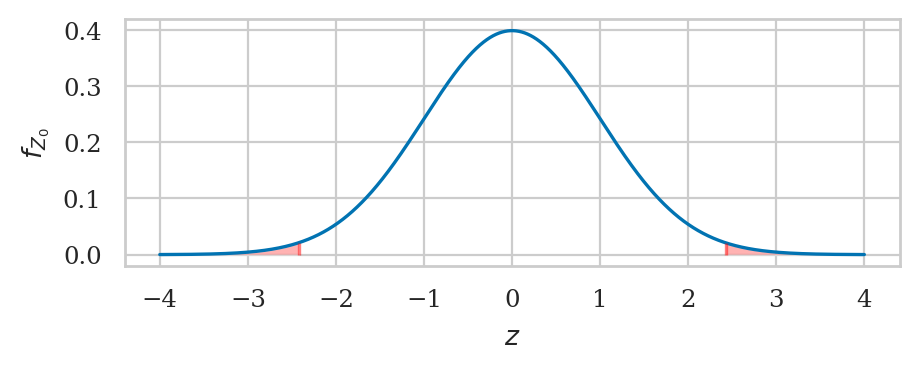
from ministats import calc_prob_and_plot_tails
_, ax = calc_prob_and_plot_tails(rvZ0, -obsz04, obsz04, xlims=[-4,4])
ax.set_title(None)
ax.set_xlabel("$z$")
ax.set_ylabel("$f_{Z_0}$");
Alternative calculation without pivotal transformation#
Note also the pivotal transformation to the standard \(Z\) is not necessary. We could have obtained the same \(p\)-value directly from the sampling distribution of the mean, which is described by a non-standard normal distribution:
from scipy.stats import norm
rvKbar0 = norm(loc=muK0, scale=se04)
#######################################################
dev = abs(obsmean04 - muK0)
dev
3.833499999999958
# left tail            +  right tail
rvKbar0.cdf(muK0-dev)  +  (1 - rvKbar0.cdf(muK0+dev))
0.015328711497996476
from ministats import calc_prob_and_plot_tails
dev = abs(obsmean04-muK0)
_, ax = calc_prob_and_plot_tails(rvKbar0, muK0-dev, muK0+dev)
ax.set_title(None)
ax.set_xlabel(r"$\overline{\mathbf{k}}$")
ax.set_ylabel(r"$f_{\overline{\mathbf{K}}_0}$");
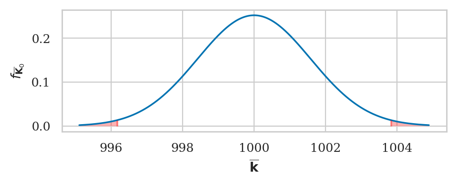
The \(p\)-value we obtain is exactly the same.
Example 2N: test for the mean of Batch 01#
kombucha = pd.read_csv("datasets/kombucha.csv")
ksample01 = kombucha[kombucha["batch"]==1]["volume"]
n01 = len(ksample01)
n01
40
# observed mean
obsmean01 = mean(ksample01)
obsmean01
999.10375
# standard error of the mean
se01 = sigmaK0 / np.sqrt(n01)
se01
1.5811388300841895
Note the standard error is the same as se04 we calculated in Example 1N.
This is because the sample size is the same,
and we’re relying on the same assumptions about the standard deviation of the theoretical distribution.
# compute the z statistic
obsz01 = (obsmean01 - muK0) / se01
obsz01
-0.5668382705851878
from scipy.stats import norm

rvZ0 = norm(loc=0, scale=1)
#          left tail               +  right tail
pvalue01 = rvZ0.cdf(-abs(obsz01))  +  (1 - rvZ0.cdf(abs(obsz01)))
pvalue01
0.5708240666473916
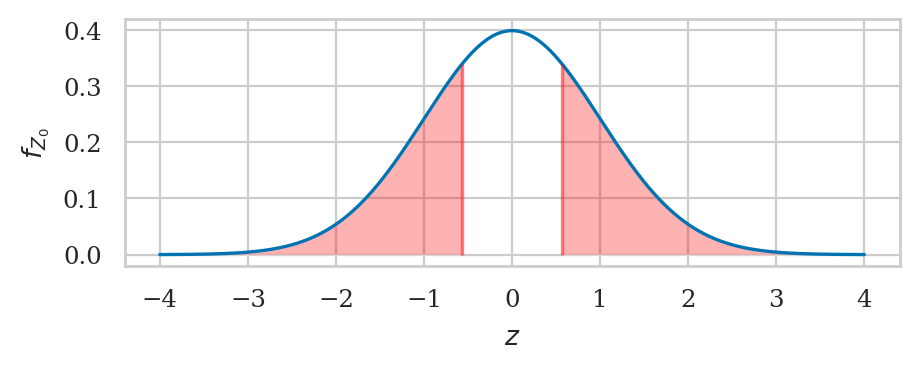
The \(p\)-value is large, so there is no reason to reject \(H_0\). We conclude that Batch 01 must be regular.
from ministats import calc_prob_and_plot_tails
_, ax= calc_prob_and_plot_tails(rvZ0, obsz01, -obsz01, xlims=[-4,4])
ax.set_title(None)
ax.set_xlabel("$z$")
ax.set_ylabel("$f_{Z_0}$");
Test for the mean (unknown variance)#
Analytical approximation based on Student’s \(t\)-distribution#
Consider again a theoretical distribution \(X_0 \sim \mathcal{N}(\mu_{X_0}, \sigma_{X_0})\), but this time assume that \(\sigma_{X_0}\) is not known.
The sampling distribution of the mean \(\overline{\mathbf{X}}_0\) for samples of size \(n\), after applying the location-scale transformation, can be modelled in terms of the standard \(t\)-distribution with \(n-1\) degrees of freedom:
Example 1T: test for the mean of Batch 04#
Assume we know mean, but not variance#
kombucha = pd.read_csv("datasets/kombucha.csv")
ksample04 = kombucha[kombucha["batch"]==4]["volume"]
n04 = len(ksample04)
n04
40
# estimated standard error of the mean
s04 = std(ksample04)
s04
7.852174139558339
sehat04 = s04 / np.sqrt(n04)
sehat04
1.24153774326386
Recall the value se04 = \(\stderr{\overline{\mathbf{k}}_{04},0}=\frac{\sigma_{K_0}}{\sqrt{40}} = 1.58\),
which we obtained by assuming the population standard deviation is known.
We see that sehat04 is an underestimate, because the sample standard deviation s04 happens to be smaller than the true population standard deviation \(\sigma_{K_0} = 10\).
# observed sample mean
obsmean04 = mean(ksample04)
obsmean04
1003.8335
# compute the t statistic
obst04 = (obsmean04 - muK0) / sehat04
obst04
3.0877031494202725
from scipy.stats import t as tdist

df04 = n04 - 1  # n-1 degrees of freedom
rvT04 = tdist(df=df04)

#           left tail          +  right tail
pvalue04t = rvT04.cdf(-obst04) +  (1-rvT04.cdf(obst04))
pvalue04t
0.0037056653503329314
# no figure because too small
Effect size estimates#
We can estimate the effect size using the formula \(\widehat{\Delta} = \overline{\mathbf{k}}_{04} - \mu_{K_0}\).
obsmean04 - muK0
3.833499999999958
We can also obtain confidence interval for the effect size \(\ci{\Delta,0.9}\) by first computing a 90% confidence interval for the population mean \(\ci{\mu,0.9}\), then subtracting theoretical mean \(\mu_{K_0}\).
from ministats import ci_mean
cimu04 = ci_mean(ksample04, alpha=0.1, method="a")
cimu04
[1001.7416639437092, 1005.9253360562907]
[cimu04[0]-muK0, cimu04[1]-muK0]
[1.7416639437092272, 5.925336056290689]
Example 2T: test for the mean of Batch 01#
kombucha = pd.read_csv("datasets/kombucha.csv")
ksample01 = kombucha[kombucha["batch"]==1]["volume"]
# estimated standard error of the mean
s01 = std(ksample01)
n01 = len(ksample01)
sehat01 = s01 / np.sqrt(n01)
sehat01
1.5446402654597249
cf. se01 = \(\stderr{\overline{\mathbf{k}}_{01},0}=\frac{\sigma_{K_0}}{\sqrt{40}} = 1.58\),
# observed sample mean
obsmean01 = mean(ksample01)
obsmean01
999.10375
# compute the t statistic
obst01 = (obsmean01 - muK0) / sehat01
obst01
-0.5802321874169595
from scipy.stats import t as tdist

df01 = n01 - 1  # n-1 degrees of freedom
rvT01 = tdist(df=df01)
#######################################################
#           left tail          +  right tail
pvalue01t = rvT01.cdf(-abs(obst01)) + 1-rvT01.cdf(abs(obst01))
pvalue01t
0.5650956637295477
# # ALT. compute right tail and double the value
# p_right = 1 - rvT01.cdf(abs(obst01))
# pvalue01t = 2 * p_right
# pvalue01t
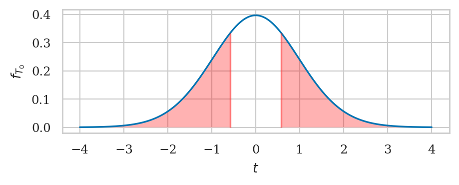
from ministats import calc_prob_and_plot_tails
_, ax = calc_prob_and_plot_tails(rvT01, obst01, -obst01, xlims=[-4,4])
ax.set_title(None)
ax.set_xlabel("$t$")
ax.set_ylabel("$f_{T_0}$");
Generic function#
from ministats import ttest_mean
%psource ttest_mean
Test for the variance#
Formula for sampling distribution of the variance#
Chi-square test for variance#
If the theoretical distribution under the null hypothesis is normal \(K_0 \sim \mathcal{N}(\mu_{K_0}, \sigma_{K_0})\), then the sampling distribution of variance for samples of size \(n\) is described by a scaled chi-square distribution:
Example 3X: test for the variance of Batch 02#
kombucha = pd.read_csv("datasets/kombucha.csv")
ksample02 = kombucha[kombucha["batch"]==2]["volume"]
n02 = len(ksample02)
n02
20
obsvar02 = var(ksample02)
obsvar02
124.31760105263139
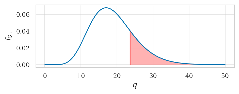
We can now compute the \(q\)-statistic, which is the observed sample variance estimate \(s_{\mathbf{k}_{02}}^2 = 124.32\) divided by the scale factor \(\tfrac{ \sigma_{K_0}^2 }{ n-1 }\).
obsq02 = (n02-1) * obsvar02 / sigmaK0**2
obsq02
23.620344199999963
from scipy.stats import chi2

rvX2 = chi2(df=n02-1)
pvalue02 = 1 - rvX2.cdf(obsq02)
pvalue02
0.21112073283603827
The \(p\)-value is large, so there is no reason to reject \(H_0\).
_, ax = calc_prob_and_plot_tails(rvX2, 0, obsq02, xlims=[0,50])
ax.set_title(None)
ax.set_xlabel("$q$")
ax.set_ylabel("$f_{Q_0}$");
Example 4X: test for the variance of Batch 08#
kombucha = pd.read_csv("datasets/kombucha.csv")
ksample08 = kombucha[kombucha["batch"]==8]["volume"]
n08 = len(ksample08)
n08
40
obsvar08 = var(ksample08)
obsvar08
169.9979220512824
obsq08 = (n08-1) * obsvar08 / sigmaK0**2
obsq08
66.29918960000013
from scipy.stats import chi2

rvX2 = chi2(df=n08-1)
pvalue08 = 1 - rvX2.cdf(obsq08)
pvalue08
0.0041211873587608805
The \(p\)-value is vary small, so we reject \(H_0\). According to our analysis based on the sample variance from Batch 08, this batch seems to be irregular: it has an abnormally large variance.
Effect size estimates#
We can estimate the effect size using the formula \(\widehat{\Delta} = s^2_{\mathbf{k}_{08}} / \sigma_{K_0}^2\).
obsvar08 / sigmaK0**2
1.699979220512824
We can also obtain confidence interval for the effect size \(\ci{\Delta,0.9}\) by first computing a 90% confidence interval for the variance \(\ci{\sigma^2,0.9}\), then dividing by the theoretical variance \(\sigma_{K_0}^2\).
from ministats import ci_var
civar08 = ci_var(ksample08, alpha=0.1, method="a")
ci_l = civar08[0] / sigmaK0**2
ci_u = civar08[1] / sigmaK0**2
[ci_l, ci_u]
[1.2148888239061655, 2.58019779302895]
Compare this to the bootstrap confidence interval for the effect size \(\ci{\Delta,0.9}^* = [1.17, 2.18]\) , which we obtained earlier in Section 3.3.
Alternative calculation methods#
Using scipy.stats.ttest_1samp for one-sample \(t\)-test#
# ALT. using existing function `scipy.stats`
from scipy.stats import ttest_1samp
res = ttest_1samp(ksample04, popmean=muK0)
res.pvalue
0.0037056653503329644
cimu04 = res.confidence_interval(confidence_level=0.9)
[cimu04.low - muK0, cimu04.high - muK0]
[1.7416639437092272, 5.925336056290689]
We see the \(p\)-value and the 90% confidence interval are same the ones we calculated earlier in Example 1T.
Bootstrap estimate of the standard error#
Another way to obtain the standard error of the mean (the standard deviation of the sampling distribution of the mean) is to use the bootstrap estimate.
See problems PNN and PMM in the notebook chapter3_problems.ipynb.
Explanations#
Helper function for calculating \(p\)-values#
def tailprobs(rvH0, obs, alt="two-sided"):
    """
    Calculate the probability of all outcomes of the random variable `rvH0`
    that are equal or more extreme than the observed value `obs`.
    """
    assert alt in ["greater", "less", "two-sided"]
    if alt == "greater":
        pvalue = 1 - rvH0.cdf(obs)
    elif alt == "less":
        pvalue = rvH0.cdf(obs)
    elif alt == "two-sided":  # assumes distribution is symmetric
        meanH0 = rvH0.mean()
        obsdev = abs(obs - meanH0)
        pleft = rvH0.cdf(meanH0 - obsdev)
        pright = 1 - rvH0.cdf(meanH0 + obsdev)
        pvalue = pleft + pright
    return pvalue
One-sided \(p\)-value calculation example#
Reusing the variables n02=20 and obsq02=23.62 we calculated in Example 3X above,
we can calculate the \(p\)-value by calling the helper function tailprobs
with the option alt="greater":
rvX2 = chi2(df=n02-1)
tailprobs(rvX2, obsq02, alt="greater")
0.21112073283603827
The value we obtained is identical to the value pvalue02 we obtained in Example 3X,
so we know the function tailprobs works as expected for \(p\)-value calculations of type (a),
where we want to detect only positive deviations from the expected distribution under \(H_0\).
Two-sided \(p\)-value calculation example#
Reusing the variable obsz04 we calculated in Example 1N above,
we can calculate the \(p\)-value by calling the function tailprobs
with the option alt="two-sided":
rvZ0 = norm(loc=0, scale=1)
tailprobs(rvZ0, obsz04, alt="two-sided")
0.015328711497996476
The value we obtained is identical to the value pvalue04 we obtained in Example 1N,
so we know the function tailprobs works as expected for \(p\)-value calculations of type (c),
where we want to detect both positive and negative deviations from the expected distribution under \(H_0\).
Discussion#
Statistical modelling and assumptions#
Exercises#
Exercise NN: use integration to obtain of the probability …#
from scipy.integrate import quad
fZ0 = rvZ0.pdf
oo = np.inf
# left tail                 +  right tail
quad(fZ0, -oo, -obsz04)[0]  +  quad(fZ0, obsz04, oo)[0]
0.015328711497995967