Section 4.4 — Regression with categorical predictors#
This notebook contains the code examples from Section 4.4 Regression with categorical predictors from the No Bullshit Guide to Statistics.
Notebook setup#
# Ensure required Python modules are installed
%pip install --quiet numpy scipy seaborn pandas statsmodels ministats
Note: you may need to restart the kernel to use updated packages.
# load Python modules
import numpy as np
import pandas as pd
import seaborn as sns
import matplotlib.pyplot as plt
import statsmodels.formula.api as smf
# Figures setup
plt.clf()  # needed otherwise `sns.set_theme` doesn't work
sns.set_theme(
    context="paper",
    style="whitegrid",
    palette="colorblind",
    rc={"font.family": "serif",
        "font.serif": ["Palatino", "DejaVu Serif", "serif"],
        "figure.figsize": (5, 1.6)},
)
%config InlineBackend.figure_format = 'retina'
<Figure size 640x480 with 0 Axes>
# Simple float __repr__
if int(np.__version__.split(".")[0]) >= 2:
    np.set_printoptions(legacy='1.25')
# Download datasets/ directory if necessary
from ministats import ensure_datasets
ensure_datasets()
datasets/ directory already exists.
Definitions#
Design matrix for linear model lm1#
students = pd.read_csv("datasets/students.csv")
lm1 = smf.ols("score ~ 1 + effort", data=students).fit()
lm1.model.exog[0:3]
array([[ 1.  , 10.96],
       [ 1.  ,  8.69],
       [ 1.  ,  8.6 ]])
students["effort"].values[0:3]
array([10.96, 8.69, 8.6 ])
Design matrix for linear model lm2#
doctors = pd.read_csv("datasets/doctors.csv")
formula = "score ~ 1 + alc + weed + exrc"
lm2  = smf.ols(formula, data=doctors).fit()
lm2.model.exog[0:3]
array([[ 1. ,  0. ,  5. ,  0. ],
       [ 1. , 20. ,  0. ,  4.5],
       [ 1. ,  1. ,  0. ,  7. ]])
doctors[["alc","weed","exrc"]].values[0:3]
array([[ 0. ,  5. ,  0. ],
       [20. ,  0. ,  4.5],
       [ 1. ,  0. ,  7. ]])
Example 1: binary predictor variable#
import statsmodels.formula.api as smf
lmloc = smf.ols("score ~ 1 + C(loc)", data=doctors).fit()
lmloc.params
Intercept        52.956522
C(loc)[T.urb]    -6.992885
dtype: float64
from ministats.plots.figures import plot_lm_ttest

with plt.rc_context({"figure.figsize":(4.6,2.2)}):
    ax = plot_lm_ttest(doctors, x="loc", y="score")
    ax.set_ylim([25,90])
    sns.move_legend(ax, "upper center")
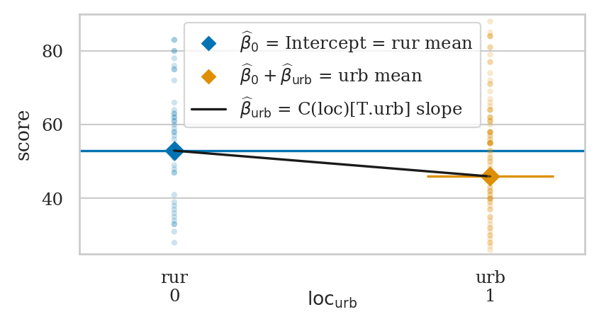
rur_mean = doctors[doctors["loc"]=="rur"]["score"].mean()
urb_mean = doctors[doctors["loc"]=="urb"]["score"].mean()

rur_mean, urb_mean, urb_mean - rur_mean
(52.95652173913044, 45.96363636363636, -6.992885375494076)
Encoding#
doctors["loc"][0:5]
0    rur
1    urb
2    urb
3    urb
4    rur
Name: loc, dtype: str
lmloc.model.exog[0:5]
array([[1., 0.],
       [1., 1.],
       [1., 1.],
       [1., 1.],
       [1., 0.]])
# ALT.
# dmatrix("1 + C(loc)", doctors)[0:5]
Dummy coding for categorical predictors#
cats = ["A", "B", "C", "C"]
catdf = pd.DataFrame({"cat":cats})
catdf
| cat | |
|---|---|
| 0 | A |
| 1 | B |
| 2 | C |
| 3 | C |
from patsy import dmatrix

dmatrix("1 + C(cat)", data=catdf)
DesignMatrix with shape (4, 3)
  Intercept  C(cat)[T.B]  C(cat)[T.C]
          1            0            0
          1            1            0
          1            0            1
          1            0            1
  Terms:
    'Intercept' (column 0)
    'C(cat)' (columns 1:3)
Example 2: predictors with three levels#
doctors = pd.read_csv("datasets/doctors.csv")
doctors["work"].head(5)
0    hos
1    cli
2    hos
3    eld
4    cli
Name: work, dtype: str
dmatrix("1 + C(work)", data=doctors)[0:5]
array([[1., 0., 1.],
       [1., 0., 0.],
       [1., 0., 1.],
       [1., 1., 0.],
       [1., 0., 0.]])
lmw = smf.ols("score ~ 1 + C(work)", data=doctors).fit()
lmw.params
Intercept         46.545455
C(work)[T.eld]     4.569930
C(work)[T.hos]     2.668831
dtype: float64

lmw.rsquared
0.0077217625749193
lmw.fvalue, lmw.f_pvalue
(0.5953116925291129, 0.5526627461285684)
Example 3: improved model for the sleep scores#
We can mix of numerical and categorical predictors
formula3 = "score ~ 1 + alc + weed + exrc + C(loc)"
lm3 = smf.ols(formula3, data=doctors).fit()
lm3.params
Intercept        63.606961
C(loc)[T.urb]    -5.002404
alc              -1.784915
weed             -0.840668
exrc              1.783107
dtype: float64
lm3.rsquared, lm3.aic
(0.8544615790287664, 1092.5985552344712)
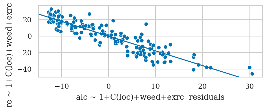
from ministats import plot_partreg

plot_partreg(lm3, "alc");
lm3.summary()
| Dep. Variable: | score | R-squared: | 0.854 |
|---|---|---|---|
| Model: | OLS | Adj. R-squared: | 0.851 |
| Method: | Least Squares | F-statistic: | 221.6 |
| Date: | Fri, 17 Jul 2026 | Prob (F-statistic): | 4.18e-62 |
| Time: | 16:50:10 | Log-Likelihood: | -541.30 |
| No. Observations: | 156 | AIC: | 1093. |
| Df Residuals: | 151 | BIC: | 1108. |
| Df Model: | 4 | ||
| Covariance Type: | nonrobust |
| coef | std err | t | P>|t| | [0.025 | 0.975] | |
|---|---|---|---|---|---|---|
| Intercept | 63.6070 | 1.524 | 41.734 | 0.000 | 60.596 | 66.618 |
| C(loc)[T.urb] | -5.0024 | 1.401 | -3.572 | 0.000 | -7.770 | -2.235 |
| alc | -1.7849 | 0.068 | -26.424 | 0.000 | -1.918 | -1.651 |
| weed | -0.8407 | 0.462 | -1.821 | 0.071 | -1.753 | 0.071 |
| exrc | 1.7831 | 0.133 | 13.400 | 0.000 | 1.520 | 2.046 |
| Omnibus: | 4.325 | Durbin-Watson: | 1.823 |
|---|---|---|---|
| Prob(Omnibus): | 0.115 | Jarque-Bera (JB): | 4.038 |
| Skew: | 0.279 | Prob(JB): | 0.133 |
| Kurtosis: | 3.556 | Cond. No. | 46.2 |
Notes:
[1] Standard Errors assume that the covariance matrix of the errors is correctly specified.
Compare to the model without loc predictor#
formula2 = "score ~ 1 + alc + weed + exrc"
lm2 = smf.ols(formula2, data=doctors).fit()
F, p, _ = lm3.compare_f_test(lm2)
F, p
(12.75811559629559, 0.0004759812308491926)
Everything is a linear model#
One-sample t-test as a linear model#
kombucha = pd.read_csv("datasets/kombucha.csv")
ksample04 = kombucha[kombucha["batch"]==4]["volume"]
ksample04.mean()
1003.8335
from scipy.stats import ttest_1samp
resk = ttest_1samp(ksample04, popmean=1000)
resk.statistic, resk.pvalue
(3.087703149420272, 0.0037056653503329644)
# # ALT. using the helper function from `ministats`
# from ministats import ttest_mean
# ttest_mean(ksample04, mu0=1000)
# Prepare zero-centered data (volume - 1000)
kdat04 = pd.DataFrame()
kdat04["zcvolume"] = ksample04 - 1000

# Fit linear model with only an intercept term
import statsmodels.formula.api as smf
lmk = smf.ols("zcvolume ~ 1", data=kdat04).fit()
lmk.params
Intercept    3.8335
dtype: float64
lmk.tvalues.iloc[0], lmk.pvalues.iloc[0]
(3.0877031494203044, 0.0037056653503326456)
Two-sample t-test as a linear model#
East vs. West electricity prices#
eprices = pd.read_csv("datasets/eprices.csv")
pricesW = eprices[eprices["loc"]=="West"]["price"]
pricesE = eprices[eprices["loc"]=="East"]["price"]
pricesW.mean() - pricesE.mean()
3.000000000000001
Two-sample t-test with pooled variance#
from scipy.stats import ttest_ind
rese = ttest_ind(pricesW, pricesE, equal_var=True)
rese.statistic, rese.pvalue
(5.022875513276465, 0.00012497067987678512)
ci_Delta = rese.confidence_interval(confidence_level=0.9)
[ci_Delta.low, ci_Delta.high]
[1.9572405258731596, 4.042759474126841]
Linear model approach#
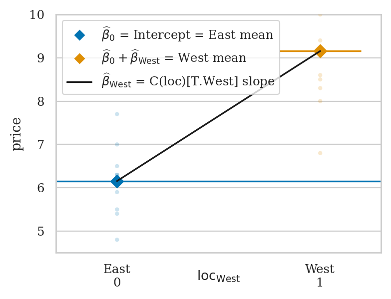
lme = smf.ols("price ~ 1 + C(loc)", data=eprices).fit()
print(lme.params)
lme.tvalues.iloc[1], lme.pvalues.iloc[1]
Intercept         6.155556
C(loc)[T.West]    3.000000
dtype: float64
(5.02287551327646, 0.0001249706798767861)
lme.conf_int(alpha=0.1).iloc[1].values
array([1.95724053, 4.04275947])
from ministats.plots.figures import plot_lm_ttest

with plt.rc_context({"figure.figsize":(4.2,3.1)}):
    ax = plot_lm_ttest(eprices, x="loc", y="price")
    ax.set_ylim([4.5,10])
    sns.move_legend(ax, "upper left")
    ax.xaxis.set_label_coords(0.5, -0.07)
Example 1 (revisited): urban vs. rural doctors#
from scipy.stats import ttest_ind

scoresR = doctors[doctors["loc"]=="rur"]["score"]
scoresU = doctors[doctors["loc"]=="urb"]["score"]

resloc = ttest_ind(scoresU, scoresR, equal_var=True)
resloc.statistic, resloc.pvalue
(-1.9657612140164198, 0.05112460353979367)
lmloc = smf.ols("score ~ 1 + C(loc)", data=doctors).fit()
lmloc.tvalues.iloc[1], lmloc.pvalues.iloc[1]
(-1.9657612140164218, 0.05112460353979346)
One-way ANOVA as a linear model#
from scipy.stats import f_oneway

scoresH = doctors[doctors["work"]=="hos"]["score"]
scoresC = doctors[doctors["work"]=="cli"]["score"]
scoresE = doctors[doctors["work"]=="eld"]["score"]

resw = f_oneway(scoresH, scoresC, scoresE)
resw.statistic, resw.pvalue
(0.5953116925291182, 0.5526627461285655)
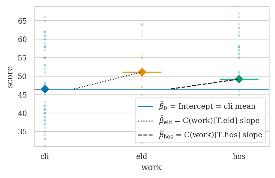
lmw = smf.ols("score ~ 1 + C(work)", data=doctors).fit()
print(lmw.params)
lmw.fvalue, lmw.f_pvalue
Intercept         46.545455
C(work)[T.eld]     4.569930
C(work)[T.hos]     2.668831
dtype: float64
(0.5953116925291129, 0.5526627461285684)
from ministats.plots.figures import plot_lm_anova

with plt.rc_context({"figure.figsize":(5,3)}):
    ax = plot_lm_anova(doctors, x="work", y="score")
    ax.set_ylim([31,69])
    sns.move_legend(ax, "lower right")
# BONUS: print ANOVA table
# import statsmodels.api as sm
# sm.stats.anova_lm(lmw)
Nonparametric tests#
One-sample Wilcoxon signed-rank test#
kombucha = pd.read_csv("datasets/kombucha.csv")
ksample04 = kombucha[kombucha["batch"]==4]["volume"]

# Zero-centered volumes
zcksample04 = ksample04 - 1000

from scipy.stats import wilcoxon
reswil = wilcoxon(zcksample04)
reswil.pvalue
0.002770629538645153
# Create a new data frame with the signed ranks of the volumes
df_zcsr = pd.DataFrame()
df_zcsr["zcvolume_sr"] = np.sign(zcksample04) * zcksample04.abs().rank()

lmwil = smf.ols("zcvolume_sr ~ 1", data=df_zcsr).fit()
lmwil.pvalues.iloc[0]
0.0022841508459744263
Mann-Whitney U-test#
scoresR = doctors[doctors["loc"]=="rur"]["score"]
scoresU = doctors[doctors["loc"]=="urb"]["score"]

from scipy.stats import mannwhitneyu
resmwu = mannwhitneyu(scoresU, scoresR)
resmwu.pvalue
0.050083369850737636
# Compute the (unsigned) ranks of the scores
doctors["score_r"] = doctors["score"].rank()

# Fit a linear model
lmmwu = smf.ols("score_r ~ 1 + C(loc)", data=doctors).fit()
lmmwu.pvalues.iloc[1]
0.049533887469988755
Kruskal-Wallis analysis of variance by ranks#
from scipy.stats import kruskal
reskw = kruskal(scoresH, scoresC, scoresE)
reskw.pvalue
0.4441051932875236
# Compute the (unsigned) ranks of the scores
doctors["score_r"] = doctors["score"].rank()

lmkw = smf.ols("score_r ~ 1 + C(work)", data=doctors).fit()
lmkw.f_pvalue
0.4468887214966093
Explanations#
Dummy coding options#
dmatrix("cat", data=catdf)
DesignMatrix with shape (4, 3)
  Intercept  cat[T.B]  cat[T.C]
          1         0         0
          1         1         0
          1         0         1
          1         0         1
  Terms:
    'Intercept' (column 0)
    'cat' (columns 1:3)
dmatrix("C(cat)", data=catdf)
DesignMatrix with shape (4, 3)
  Intercept  C(cat)[T.B]  C(cat)[T.C]
          1            0            0
          1            1            0
          1            0            1
          1            0            1
  Terms:
    'Intercept' (column 0)
    'C(cat)' (columns 1:3)
dmatrix("C(cat, Treatment)", data=catdf)
DesignMatrix with shape (4, 3)
  Intercept  C(cat, Treatment)[T.B]  C(cat, Treatment)[T.C]
          1                       0                       0
          1                       1                       0
          1                       0                       1
          1                       0                       1
  Terms:
    'Intercept' (column 0)
    'C(cat, Treatment)' (columns 1:3)
dmatrix("C(cat, Treatment('B'))", data=catdf)
# ALT. dmatrix("C(cat, Treatment(1))", data=catdf)
DesignMatrix with shape (4, 3)
  Intercept  C(cat, Treatment('B'))[T.A]  C(cat, Treatment('B'))[T.C]
          1                            1                            0
          1                            0                            0
          1                            0                            1
          1                            0                            1
  Terms:
    'Intercept' (column 0)
    "C(cat, Treatment('B'))" (columns 1:3)
Avoiding perfect collinearity#
df_col = pd.DataFrame()
df_col["iscli"] = (doctors["work"] == "cli").astype(int)
df_col["iseld"] = (doctors["work"] == "eld").astype(int)
df_col["ishos"] = (doctors["work"] == "hos").astype(int)
df_col["score"] = doctors["score"]
formula_col = "score ~ 1 + iscli + iseld + ishos"
lm_col = smf.ols(formula_col, data=df_col).fit()
lm_col.params
Intercept    36.718781
iscli         9.826673
iseld        14.396603
ishos        12.495504
dtype: float64
lm_col.condition_number
4594083276761821.0
lm2.params
Intercept    60.452901
alc          -1.800101
weed         -1.021552
exrc          1.768289
dtype: float64
Discussion#
Other coding strategies for categorical variables#
dmatrix("0 + C(cat)", data=catdf)
DesignMatrix with shape (4, 3)
  C(cat)[A]  C(cat)[B]  C(cat)[C]
          1          0          0
          0          1          0
          0          0          1
          0          0          1
  Terms:
    'C(cat)' (columns 0:3)
dmatrix("1 + C(cat, Sum)", data=catdf)
DesignMatrix with shape (4, 3)
  Intercept  C(cat, Sum)[S.A]  C(cat, Sum)[S.B]
          1                 1                 0
          1                 0                 1
          1                -1                -1
          1                -1                -1
  Terms:
    'Intercept' (column 0)
    'C(cat, Sum)' (columns 1:3)
dmatrix("1+C(cat, Diff)", data=catdf)
DesignMatrix with shape (4, 3)
  Intercept  C(cat, Diff)[D.A]  C(cat, Diff)[D.B]
          1           -0.66667           -0.33333
          1            0.33333           -0.33333
          1            0.33333            0.66667
          1            0.33333            0.66667
  Terms:
    'Intercept' (column 0)
    'C(cat, Diff)' (columns 1:3)
dmatrix("C(cat, Helmert)", data=catdf)
DesignMatrix with shape (4, 3)
  Intercept  C(cat, Helmert)[H.B]  C(cat, Helmert)[H.C]
          1                    -1                    -1
          1                     1                    -1
          1                     0                     2
          1                     0                     2
  Terms:
    'Intercept' (column 0)
    'C(cat, Helmert)' (columns 1:3)
Exercises#
EXX: redo comparison of debate and lectures scores#
students = pd.read_csv("datasets/students.csv")
lmcu = smf.ols("score ~ 1 + C(curriculum)", data=students).fit()
lmcu.tvalues.iloc[1], lmcu.pvalues.iloc[1]
(-1.7197867420465667, 0.10917234443214374)
EXX: model comparison#
formula3w = "score ~ 1 + alc + weed + exrc + C(loc) + C(work)"
lm3w = smf.ols(formula3w, data=doctors).fit()

formula3 = "score ~ 1 + alc + weed + exrc + C(loc)"
lm3 = smf.ols(formula3, data=doctors).fit()

lm3w.compare_f_test(lm3)
(1.5158185269522875, 0.22299549360240745, 2.0)
The result is non-significant which means including the predictor C(work)
in the model is not useful.
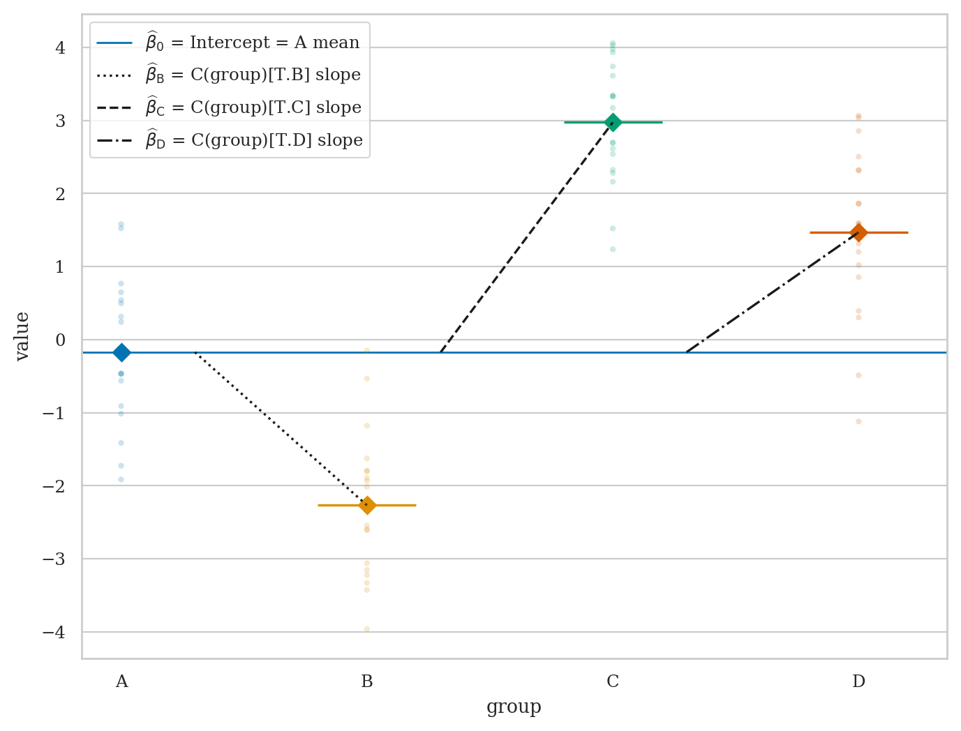
EXX: run ANOVA test#
# Construct data as a pd.DataFrame
np.random.seed(42)
As = np.random.normal(0, 1, 20)
Bs = np.random.normal(-2, 1, 20)
Cs = np.random.normal(3, 1, 20)
Ds = np.random.normal(1.5, 1, 20)

dfABCD = pd.DataFrame()
dfABCD["group"] = ["A"]*20 + ["B"]*20 + ["C"]*20 + ["D"]*20
dfABCD["value"] = np.concatenate([As, Bs, Cs, Ds])

with plt.rc_context({"figure.figsize":(8,6)}):
    ax = plot_lm_anova(dfABCD, x="group", y="value")

from scipy.stats import f_oneway
resABCD = f_oneway(As, Bs, Cs, Ds)
print(resABCD.statistic, resABCD.pvalue)

lmabcd =  smf.ols("value ~ C(group)", data=dfABCD).fit()
lmabcd.fvalue, lmabcd.f_pvalue
107.22963883851017 3.091116115443279e-27
(107.22963883851006, 3.091116115443411e-27)
Links#
Patsy and Statsmodels https://www.youtube.com/watch?v=iEANEcWqAx4
Tests as LMs: https://lindeloev.github.io/tests-as-linear/
https://danielroelfs.com/blog/everything-is-a-linear-model/ via HN