Section 2.6 — Inventory of continuous distributions#
This notebook contains all the code examples from Section 2.6 Inventory of continuous distributions of the No Bullshit Guide to Statistics.
Notebook setup#
# Ensure required Python modules are installed
%pip install --quiet numpy scipy seaborn ministats
Note: you may need to restart the kernel to use updated packages.
# load Python modules
import numpy as np
import seaborn as sns
import matplotlib.pyplot as plt
from ministats import plot_pdf
from ministats import plot_cdf
from ministats import plot_pdf_and_cdf
# Figures setup
plt.clf()  # needed otherwise `sns.set_theme` doesn't work
sns.set_theme(
    context="paper",
    style="whitegrid",
    palette="colorblind",
    rc={"font.family": "serif",
        "font.serif": ["Palatino", "DejaVu Serif", "serif"],
        "figure.figsize": (6,2)},
)
%config InlineBackend.figure_format = "retina"
<Figure size 640x480 with 0 Axes>
# Simple float __repr__
import numpy as np
if int(np.__version__.split(".")[0]) >= 2:
    np.set_printoptions(legacy='1.25')

# Set random seed for repeatability
np.random.seed(42)
Uniform distribution#
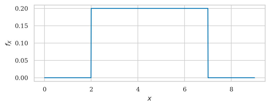
The uniform distribution \(\mathcal{U}(\alpha,\beta)\) is described by the following probability density function:
For a uniform distribution \(\mathcal{U}(\alpha,\beta)\), each \(x\) between \(\alpha\) and \(\beta\) is equally likely to occur, and values of \(x\) outside this range have zero probability of occurring.
from scipy.stats import uniform
alpha = 2
beta = 7
rvU = uniform(alpha, beta-alpha)
# draw 10 random samples from X
rvU.rvs(10)
array([3.87270059, 6.75357153, 5.65996971, 4.99329242, 2.7800932 ,
       2.7799726 , 2.29041806, 6.33088073, 5.00557506, 5.54036289])
plot_pdf(rvU, xlims=[0,9]);
# # ALT. use sns.lineplot
# # plot the probability density function (pdf) of the random variable X
# xs = np.linspace(0, 10, 1000)
# fUs = rvU.pdf(xs)
# sns.lineplot(x=xs, y=fUs)
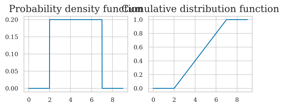
Cumulative distribution function#
plot_pdf_and_cdf(rvU, xlims=[0,9]);
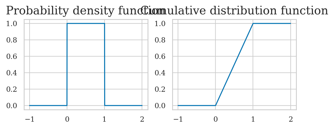
Standard uniform distribution#
The standard uniform distribution \(U_s \sim \mathcal{U}(0,1)\) is described by the following probability density function:
where \(U\) is the name of the random variable and \(u\) are particular values it can take on.
The above equation describes tells you how likely it is to observe \(\{U_s=x\}\). For a uniform distribution \(\mathcal{U}(0,1)\), each \(x\) between 0 and 1 is equally likely to occur, and values of \(x\) outside this range have zero probability of occurring.
from scipy.stats import uniform

rvUs = uniform(0, 1)
# draw 10 random samples from X
rvUs.rvs(1)
array([0.02058449])
import random

random.seed(3)
random.random()
0.23796462709189137
random.uniform(0,1)
0.5442292252959519
import numpy as np
np.random.seed(42)
np.random.rand(10)
array([0.37454012, 0.95071431, 0.73199394, 0.59865848, 0.15601864,
       0.15599452, 0.05808361, 0.86617615, 0.60111501, 0.70807258])
plot_pdf_and_cdf(rvUs, xlims=[-1,2]);
Simulating other random variables#
We can use the uniform random variable to generate random variables from other distributions.
For example,
suppose we want to generate observations of a coin toss random variable
which comes out heads 50% of the time and tails 50% of the time.
We can use the standard uniform random variables obtained from random.random()
and split the outcomes at the “halfway point” of the sample space,
to generate the 50-50 randomness of a coin toss.
The function flip_coin defined below shows how to do this:
def flip_coin():
    u = random.random()  # random number in [0,1]
    if u < 0.5:
        return "heads"
    else:
        return "tails"
# simulate one coin toss
flip_coin()
'heads'
# simulate 10 coin tosses
[flip_coin() for i in range(0,10)]
['tails',
 'tails',
 'heads',
 'heads',
 'tails',
 'heads',
 'heads',
 'tails',
 'heads',
 'tails']
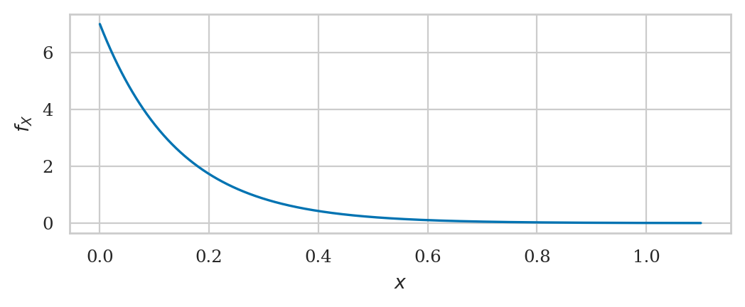
Exponential distribution#
from scipy.stats import expon

lam = 7
rvE = expon(loc=0, scale=1/lam)
To create the model rvE,
we had to specify a location parameter loc,
which we set to zero,
and a scale parameter,
which we set to the inverse of the rate parameter \(\lambda = \texttt{lam}\).
The location parameter can be used to shift the exponential distribution to the right,
but we set loc=0 to get the simple case that corresponds to the un-shifted distribution \(\textrm{Expon}(\lambda)\).
rvE.mean(), rvE.var()
(0.14285714285714285, 0.02040816326530612)
# math formulas for mean and var
1/lam, 1/lam**2
(0.14285714285714285, 0.02040816326530612)
## ALT. we can obtain mean and ver using the .stats() method
##      The code below also computes the skewness and the kurtosis
# mean, var, skew, kurt = rvE.stats(moments='mvsk')
# mean, var, skew, kurt
# f_E(5) = pdf value at x=10
rvE.pdf(0.2)
1.7261787475912451
plot_pdf(rvE, xlims=[0,1.1]);
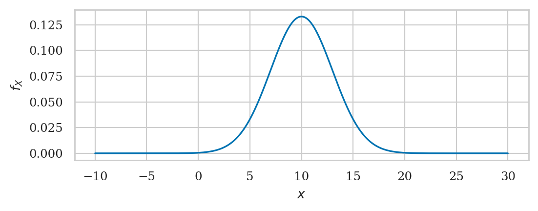
Normal distribution#
A random variable \(N\) with a normal distribution \(\mathcal{N}(\mu,\sigma)\) is described by the probability density function:
The mean \(\mu\) and the standard deviation \(\sigma\) are called the parameters of the distribution. The math notation \(\mathcal{N}(\mu, \sigma)\) is used to describe the whole family of normal probability distributions.
from scipy.stats import norm

mu = 10    # = 𝜇   where is the centre?
sigma = 3  # = 𝜎   how spread out is it?

rvN = norm(mu, sigma)
rvN.mean(), rvN.var()
(10.0, 9.0)
plot_pdf(rvN, xlims=[-10,30]);
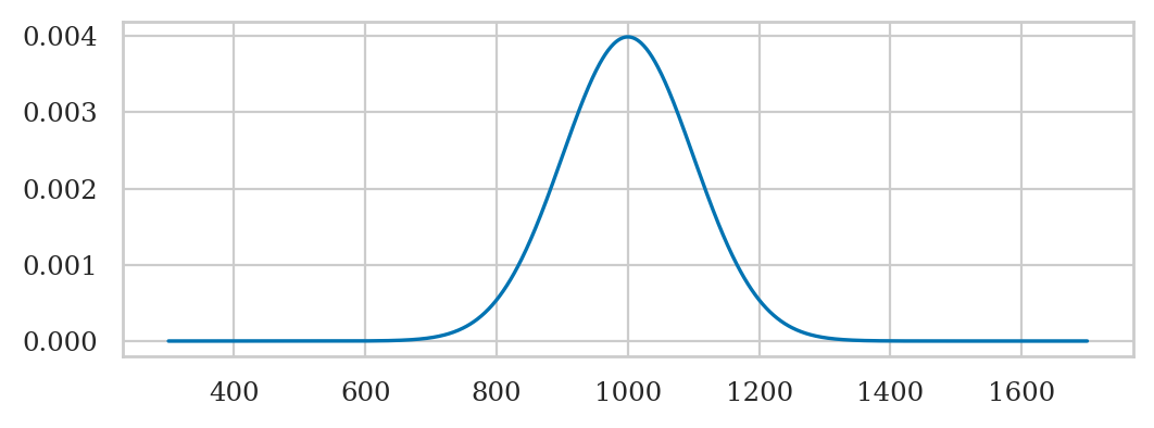
# ALT. generate the plot manually

# create a normal random variable
from scipy.stats import norm
mean = 1000   # 𝜇 (mu)    = where is its center?
std = 100     # 𝜎 (sigma) = how spread out is it?
rvN = norm(mean, std)

# plot its probability density function (pdf)
xs = np.linspace(300, 1700, 1000)
ys = rvN.pdf(xs)
ax = sns.lineplot(x=xs, y=ys)
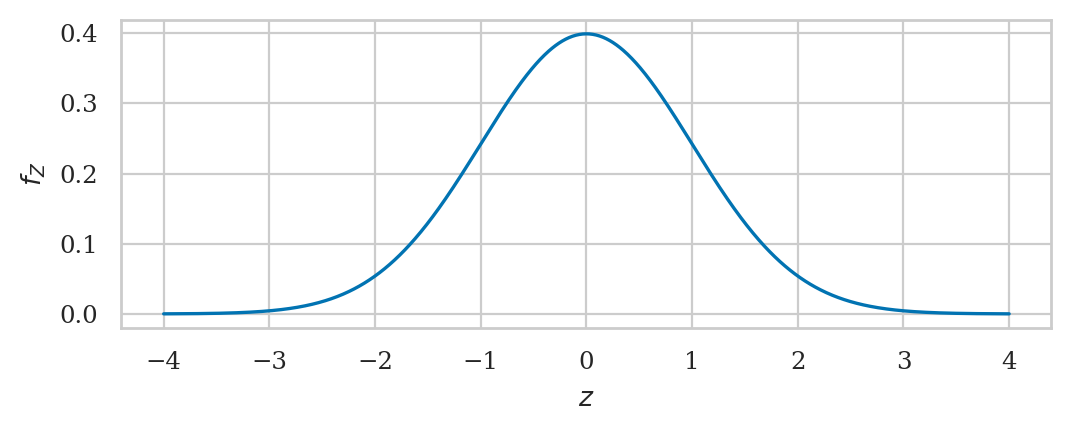
Standard normal distribution#
A standard normal is denoted \(Z\) with a normal distribution \(\mathcal{N}(\mu=0,\sigma=1)\) and described by the probability density function:
from scipy.stats import norm

rvZ = norm(0,1)
rvZ.mean(), rvZ.var()
(0.0, 1.0)
plot_pdf(rvZ, xlims=[-4,4], rv_name="Z");
Cumulative probabilities in the tails#
Probability of \(Z\) being smaller than \(-2.2\).
rvZ.cdf(-2.3)
0.010724110021675809
Probability of \(Z\) being greater than \(2.2\).
1 - rvZ.cdf(2.3)
0.010724110021675837
Probability of \(|Z| > 2.2\).
rvZ.cdf(-2.3) + (1-rvZ.cdf(2.3))
0.021448220043351646
norm.cdf(-2.3,0,1) + (1-norm.cdf(2.3,0,1))
0.021448220043351646
Inverse cumulative distribution calculations#
rvZ.ppf(0.05)
-1.6448536269514729
rvZ.ppf(0.95)
1.6448536269514722
rvZ.interval(0.9)
(-1.6448536269514729, 1.6448536269514722)
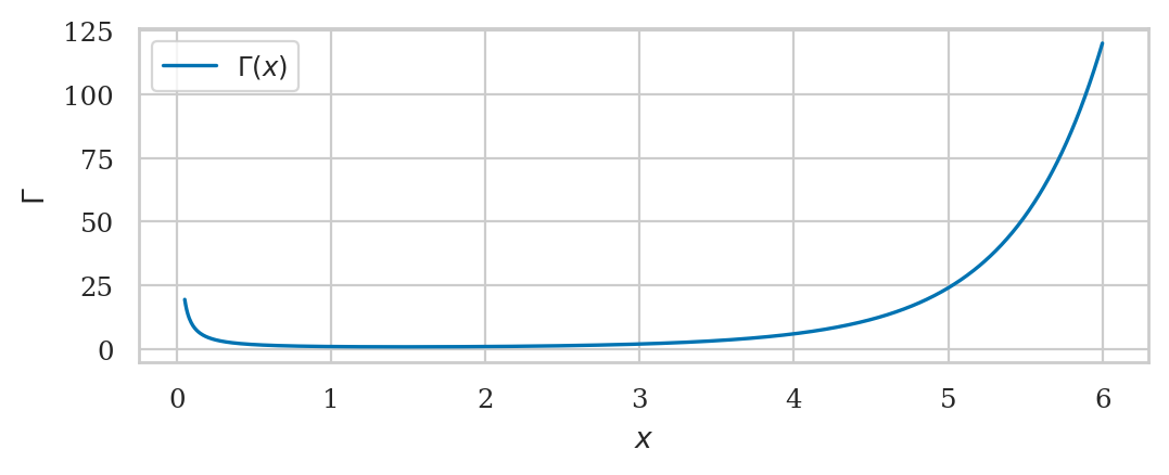
Mathematical interlude: the gamma function#
Gamma function#
from math import factorial
from scipy.special import gamma as gammaf

gammaf(1), factorial(0) # = 0! = 1
(1.0, 1)
gammaf(2), factorial(1) # = 1! = 1
(1.0, 1)
gammaf(3), factorial(2) # = 2! = 2*1
(2.0, 2)
gammaf(4), factorial(3) # = 3! = 3*2*1
(6.0, 6)
gammaf(5), factorial(4) # = 4! = 4*3*2*1
(24.0, 24)
factorial(4.1)
---------------------------------------------------------------------------
TypeError                                 Traceback (most recent call last)
Cell In[46], line 1
----> 1 factorial(4.1)

TypeError: 'float' object cannot be interpreted as an integer
gammaf(5.1)
27.93175373836837
[gammaf(x) for x in [5, 5.1, 5.2, 5.5, 5.8, 5.9, 6]]
[24.0,
 27.93175373836837,
 32.578096050331354,
 52.34277778455352,
 85.6217375127053,
 101.27019121310353,
 120.0]
# plot gammaf between 0 and 5
xs = np.linspace(0.05, 6, 1000)
fXs = gammaf(xs)

ax = sns.lineplot(x=xs, y=fXs, label="$\\Gamma(x)$")
ax.set_xlabel("$x$")
ax.set_ylabel(r"$\Gamma$")
Text(0, 0.5, '$\\Gamma$')
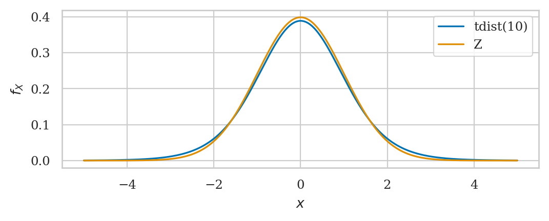
Student’s t-distribution#
This is a generalization of the standard normal with “heavy” tails.
from scipy.stats import t as tdist

rvT = tdist(df=10)
ax = plot_pdf(rvT, xlims=[-5,5], label=f"tdist(10)")
plot_pdf(rvZ, xlims=[-5,5], ax=ax, label="Z");
rvT.mean(), rvT.var()
(0.0, 1.25)
# Kurtosis formula  kurt(rvT) = 6/(df-4) for df>4
rvT.stats("k")
1.0
rvT.cdf(-2.3)
0.022127156642143573
rvT.ppf(0.05), rvT.ppf(0.95)
(-1.812461122811676, 1.8124611228116756)
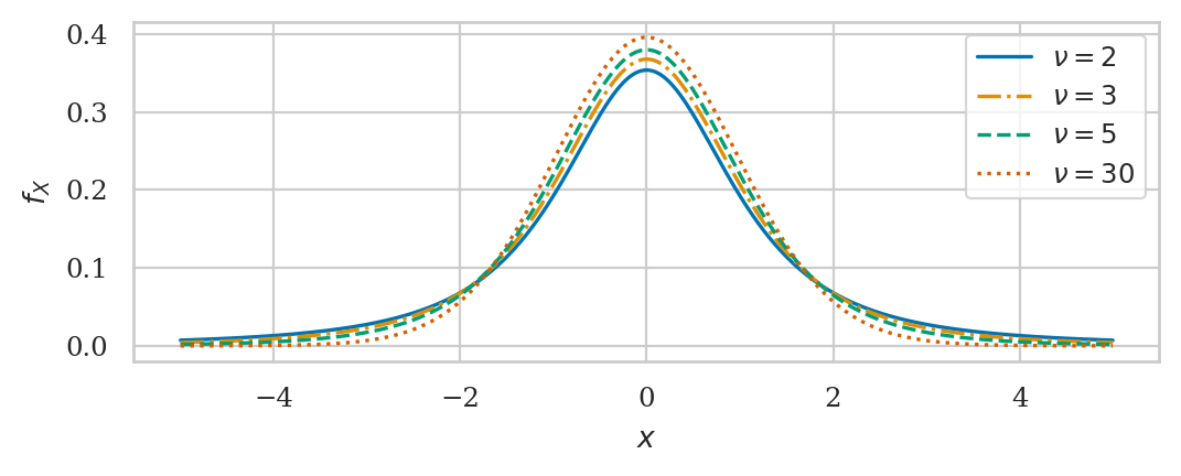
fig, ax = plt.subplots()

linestyles = ['solid', 'dashdot', 'dashed', 'dotted']

for i, df in enumerate([2,3,5,30]):
    rvT = tdist(df)
    linestyle = linestyles[i]
    plot_pdf(rvT, xlims=[-5,5], ax=ax, label="$\\nu={}$".format(df), linestyle=linestyle)
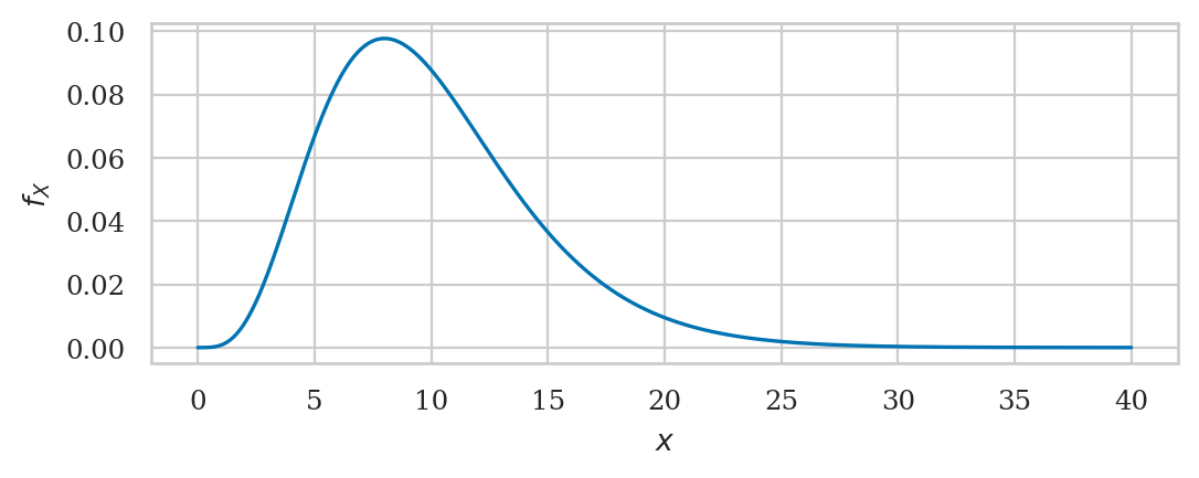
Chi-squared distribution#
from scipy.stats import chi2

df = 10
rvX2 = chi2(df)
rvX2.mean(), rvX2.var()
(10.0, 20.0)
1 - rvX2.cdf(20)
0.02925268807696113
plot_pdf(rvX2, xlims=[0,40]);
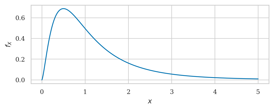
Fisher–Snedecor’s F-distribution#
from scipy.stats import f as fdist

df1, df2 = 5, 10
rvF = fdist(df1, df2)
rvF.mean(), rvF.var()
(1.25, 1.3541666666666667)
plot_pdf(rvF, xlims=[0,5]);
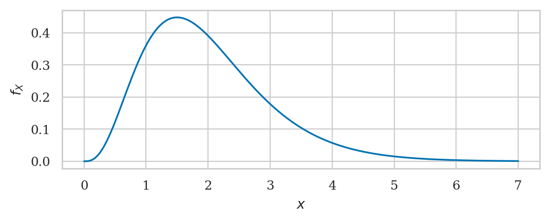
Gamma distribution#
https://en.wikipedia.org/wiki/Gamma_distribution
https://docs.scipy.org/doc/scipy/reference/generated/scipy.stats.gamma.html
from scipy.stats import gamma as gammadist

alpha = 4
loc = 0
lam = 2
beta = 1/lam

rvG = gammadist(alpha, loc, beta)
rvG.mean(), rvG.var()
(2.0, 1.0)
plot_pdf(rvG, xlims=[0,7]);
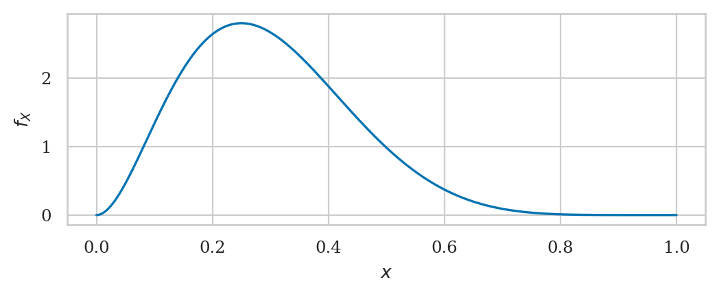
Beta distribution#
from scipy.stats import beta as betadist

alpha = 3
beta = 7

rvB = betadist(alpha, beta)
rvB.mean(), rvB.var()
(0.3, 0.019090909090909092)
plot_pdf(rvB, xlims=[0,1]);
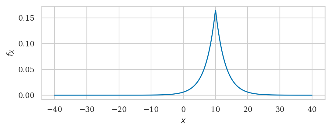
Laplace distribution#
from scipy.stats import laplace

mu = 10
b = 3
rvL = laplace(mu, b)
rvL.mean(), rvL.var()
(10.0, 18.0)
plot_pdf(rvL, xlims=[-40,40]);
Explanations#
Location-scale families#
Normal location-scale family example#
Exam question 1:#
b = 109

muN = 100
sigmaN = 5

# standardize b
z_b = (b - muN) / sigmaN
z_b
1.8
from scipy.stats import norm

rvZ = norm(loc=0, scale=1)
1 - rvZ.cdf(z_b)
0.03593031911292577
Exam question 2:#
z_l = rvZ.ppf(0.05)
z_u = rvZ.ppf(0.95)
[sigmaN*z_l + muN, sigmaN*z_u + muN]
[91.77573186524263, 108.22426813475737]
Equivalent calculations using “custom” model#
b = 109

rvN = norm(loc=100, scale=5)
1 - rvN.cdf(b)
0.03593031911292577
[rvN.ppf(0.05), rvN.ppf(0.95)]
[91.77573186524263, 108.22426813475737]
Student’s t location-scale family#
b = 109

locS = 100
scaleS = 5

t_b = (b - locS) / scaleS
t_b
1.8
from scipy.stats import t as tdist

rvT = tdist(df=6, loc=0, scale=1)
1 - rvT.cdf(t_b)
0.06097621069194403
Equivalent calculations using “custom” model#
rvS = tdist(df=6, loc=100, scale=5)

1 - rvS.cdf(b)
0.06097621069194403
Uniform location-scale family#
locV = 100
scaleV = 20

b = 115
u_b = (b - locV) / scaleV
u_b
0.75
from scipy.stats import uniform

rvU = uniform(0, 1)
1 - rvU.cdf(u_b)
0.25
rvV = uniform(100, 20)
1 - rvV.cdf(115)
0.25
Chi-square scale family#
scaleS = 10

b = 150
q_b = 150 / scaleS

from scipy.stats import chi2
rvQ = chi2(df=7)
1 - rvQ.cdf(q_b)
0.03599940476342878
rvS = chi2(df=7, scale=10)

1 - rvS.cdf(150)
0.03599940476342878
Discussion#
Relations between distributions#
SEE BOOK
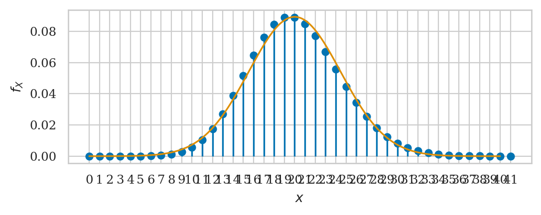
Continuity correction#
from scipy.stats import poisson
from ministats import plot_pmf
rvH = poisson(20)
ax = plot_pmf(rvH)

rvN = norm(20, np.sqrt(20))
plot_pdf(rvN, xlims=[0,40], ax=ax);
# TODO: example