Bootstrap estimation#
Click here to run the notebook interactively, so you can play with the code examples.
Notebook setup#
# Install stats library
%pip install --quiet ministats
Note: you may need to restart the kernel to use updated packages.
# Figures setup
import matplotlib.pyplot as plt
import seaborn as sns

plt.clf()  # needed otherwise `sns.set_theme` doesn't work
sns.set_theme(
    style="whitegrid",
    rc={'figure.figsize': (4, 3)},
)
# High-resolution figures please
%config InlineBackend.figure_format = 'retina'

def savefig(fig, filename, **kwargs):
    fig.tight_layout(**kwargs)
    fig.savefig(filename, dpi=300, bbox_inches="tight", pad_inches=0)
<Figure size 640x480 with 0 Axes>
Introduction#
In this notebook, I want to introduce you to some core statistics concepts from a computational perspective. By writing simple Python code (mostly for loops), you can understand some core ideas of statistics. If you’re not familiar with Python at all, I recommend you read Part 1 of the blog post series and the associated notebook first.
TL;DR My main realization from working on the STATS book is that the hands-on computational approach to statistical calculations makes learning concepts much more straightforward, as compared to the classical way of teaching which is based on formulas and procedures. This is why we’ll present the key ideas using Python code and visualizations, which should be accessible to most readers.
The statistical analyses examples in this notebook are taken from the textbook No Bullshit Guide to Stats, which you can check out if you want to learn more statistics.
Let’s start with what this is all about…
Statistical inference#
TODO: improt short version from simulation_hypothesis_tests.ipynb
The modern statistics curriculum#
There is a growing movement in statistics called “modern statistics” that puts the focus on using computers for statistical calculations. Taking a computational approach to statistics makes the material much easier to understand, because it doesn’t require memorizing any complicated formulas and procedures. Instead statistics analysis takes on a much more direct approach. The only technical requirement for understanding “modern statistics” is to know how the Python for loop works: the idea of repeating some procedure multiple times (thousands or tens of thousands of times).
Historically, part of the difficulty of learning statistics is due to the limited computation capabilities that were available when statistics was initially developed. Using a modern computational approach makes all the “hard” topics in statistics much easier to understand and allows us to focus on the big-picture ideas, instead of trying to memorize recipes and use formulas blindly. Adopting the computation approach based on Python code allows us to do a much deeper and more thorough study of statistics material.
The two techniques from the modern statistics curriculum are:
Simulation: Direct computational approach for doing probability calculations by simulating tens of thousands of samples from the relevant population. We can then calculate relevant quantities directly from the samples instead of using math formulas.
Resampling methods: This is an umbrella term for various clever techniques that reuse data from observed sample to simulate the variability in the population. We’ll talk about bootstrap estimation in this notebook.
The simulation and resampling methods are computationally expensive, but they apply for any distribution and allows us to compute any quantity of interest—not just quantities for which statisticians have found formulas.
Bootstrap estimation#
The bootstrap procedure is a powerful technique for estimating the variability of any estimator.
Computationally, the bootstrap method involves a simple for-loop that repeatedly generates new samples from the existing data. This approach to uncertainty estimation is very intuitive, and it allows us to reach a deeper understanding than the classical formulas-based approximation methods that are taught in most STATS101 courses.
Example data analysis scenario#
We’ll use an example to ground the discussions in the rest of the notebook.
IQ scores population#
This population is unknown to the person doing the analysis, but for the sake of graphs, we will pretend we’re omniscient and know what it is.
from scipy.stats import norm

muX = 108.25
rvX = norm(loc=muX, scale=15)
print(f"N(mu={muX},sigma=15)")
N(mu=108.25,sigma=15)
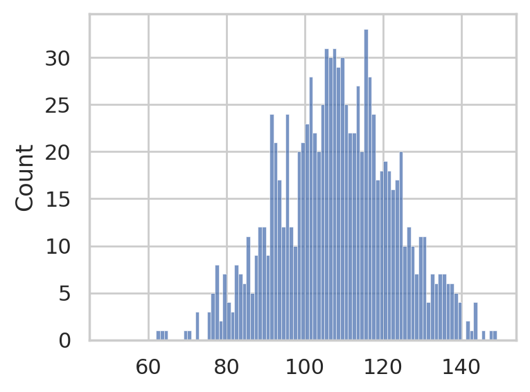
To avoid talking about models in the presentation, we make the population a concrete set of 1000 individual IQ scores.
import numpy as np
np.random.seed(43)

N = 1000
population = rvX.rvs(N)

sns.histplot(population, bins=range(50,150,1))

savefig(plt.gcf(), "figures/histplot_iqs_pop.png");
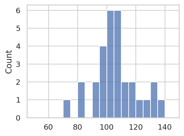
IQ scores sample#
Consider the following dataset, which consists of IQ scores of 30 students. The IQ scores are recorded in the following list.
sample = [ 95.7, 100.1,  95.3, 100.7, 123.5, 119.4,  84.4, 109.6,
          108.7,  84.7, 111.0,  92.1, 138.4, 105.2,  97.5, 115.9,
          104.4, 105.6, 104.8, 110.8,  93.8, 106.6,  71.3, 130.6,
          125.7, 130.2, 101.2, 109.0, 103.8,  96.7]
n = len(sample)
n
30
import seaborn as sns
sns.histplot(sample, bins=range(50,150,5));
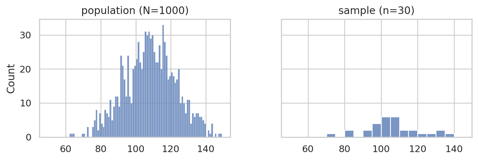
Statistical inference tasks#
with plt.rc_context({"figure.figsize":(8,2.8)}):
    fig, (ax1,ax2) = plt.subplots(1,2, sharey=True)
    # population
    sns.histplot(population, bins=np.arange(50,150,1), ax=ax1)
    ax1.set_title("population (N=1000)")
    # sample
    sns.histplot(sample, bins=range(50,150,5), ax=ax2)
    ax2.set_title("sample (n=30)")
    savefig(plt.gcf(), "figures/histplots_iqs_pop_and_sample.png", w_pad=5)
Estimation (TASK1)#
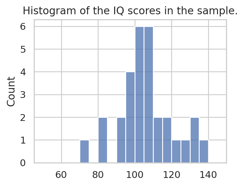
Histogram#
The first thing we often do is to produce a histogram of the data as shown below.
ax = sns.histplot(sample, bins=range(50,150,5))
ax.set_title("Histogram of the IQ scores in the sample.");
Descriptive statistics#
We can also compute the sample mean and sample standard deviation, which are the two most common descriptive statistics we can obtain for numerical data.
Sample mean#
The sample mean is defined as \(\overline{\mathbf{x}} = \tt{mean}([x_1,x_2,\ldots,x_n]) = \tfrac{1}{n}\sum_{i=1}^n x_{i}\), and corresponds to the average value.
Note we use boldface symbols to denote the whole sample \(\mathbf{x} = [x_1,x_2,\ldots,x_n]\).
def mean(xs):
    return sum(xs)/len(xs)
mean(sample)
105.89
The sample mean is an estimate for the pupulation mean \(\mu\).
Sample standard deviation#
The standard deviation is defined as \(s_{\mathbf{x}} = \tt{std}([x_1,x_2,\ldots,x_n]) = \sqrt{\tfrac{1}{n-1}\sum_{i=1}^{n}(x_i - \overline{\mathbf{x}})^2 }\).
REPEATS
Here is another estimator, the standard deviation \(s_{\mathbf{x}} = \tt{std}(\mathbf{x}) = \sqrt{ \frac{1}{n-1}\sum_{i=1}^n (x_i-\overline{\mathbf{x}})^2 }\).
import numpy as np

def std(xs):
    n = len(xs)
    xbar = mean(xs)
    s2 = sum([(xi-xbar)**2 for xi in xs])
    return np.sqrt(s2 / (n-1))
std(sample)
np.float64(14.658229417469641)
The sample standard deviation is an estimate for the population standard deviation \(\sigma\).
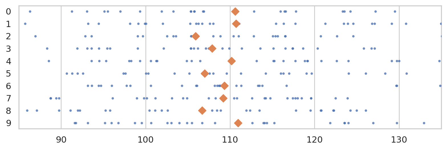
Sampling distribution of the mean#
Consider the following ten random samples from the population.
np.random.seed(5)

rsamples = []
for i in range(10):
    rsample = np.random.choice(population, n)
    rsamples.append(rsample)

with plt.rc_context({"figure.figsize":(8,2.8)}):
    ax = sns.stripplot(rsamples, orient="h", s=3, color="C0", alpha=0.8, jitter=0)
    ax.set_xlim([85,135])
    for i, rsample in enumerate(rsamples):
        rmean = np.mean(rsample)
        ax.scatter(rmean, i, marker="D", s=45, color="C1", zorder=10)

savefig(plt.gcf(), "figures/samples_from_population_n30.png")
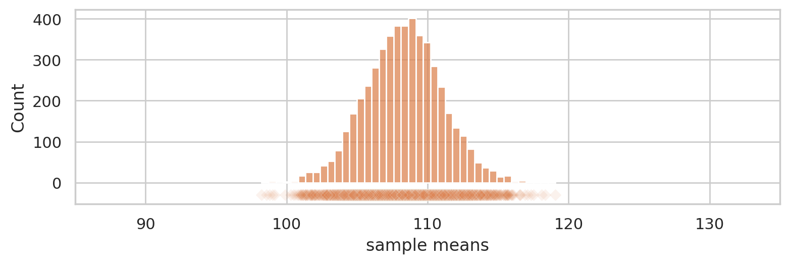
Let’s see the means from 5000 samples.
np.random.seed(6)

rmeans = []
for i in range(5000):
    rsample = np.random.choice(population, n)
    rmean = mean(rsample)
    rmeans.append(rmean)
with plt.rc_context({"figure.figsize":(8,2.8)}):
    ax = sns.histplot(rmeans, color="C1", bins=40)
    ax.set_xlim([85,135])
    sns.scatterplot(x=rmeans, y=-30, color="C1", marker="D", alpha=0.1, ax=ax)
    ax.set_ylabel("Count")
    ax.set_xlabel("sample means")
    savefig(plt.gcf(), "figures/true_sampling_dist_mean_population_n30.png")
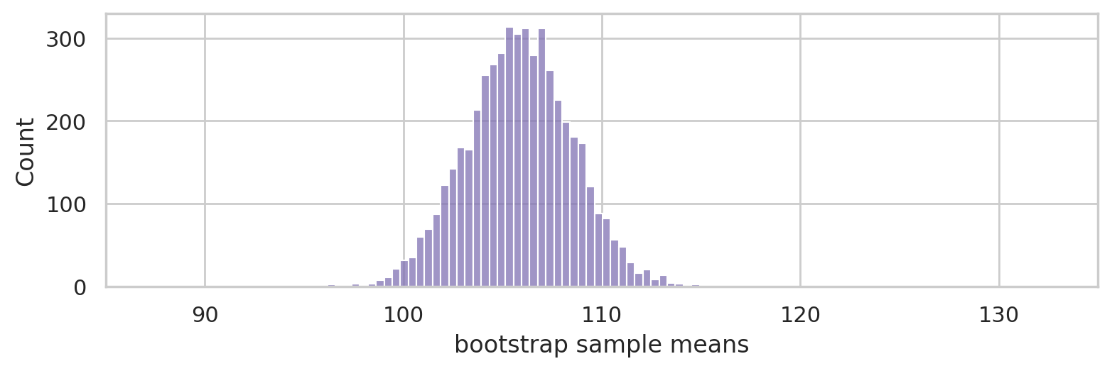
Bootstrap estimation#
Generate 5000 bootstrap samples (sampling with replacement) from the sample sample.
Use the bootstrap samples to approximate the sampling distribution of the mean.
np.random.seed(46)

bmeans = []
for i in range(5000):
    bsample = np.random.choice(sample, n)
    bmean = mean(bsample)
    bmeans.append(bmean)
with plt.rc_context({"figure.figsize":(8,2.8)}):
    ax = sns.histplot(bmeans, color="C4")
    ax.set_xlim([85,135])
    ax.set_ylim([0,330])
    ax.set_ylabel("Count")
    ax.set_xlabel("bootstrap sample means")
    savefig(plt.gcf(), "figures/bootstrap_dist_mean_iqs.png")
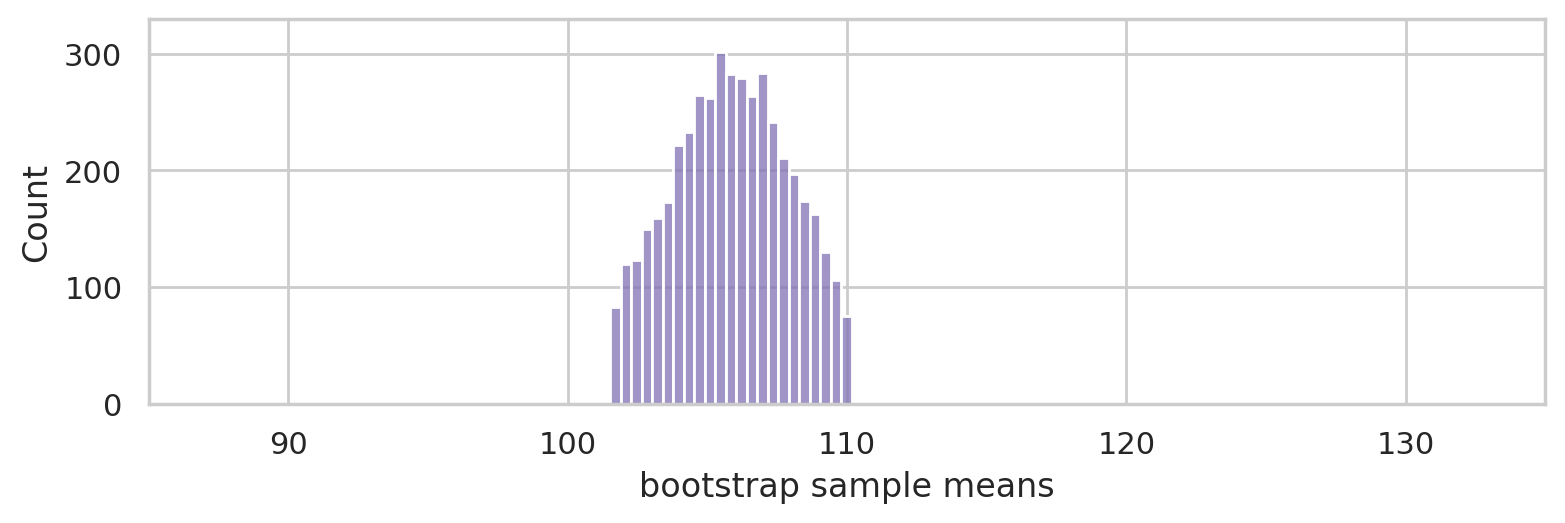
ci90 = np.percentile(bmeans, [5, 95])
ci90.round(2)
array([101.52, 110.16])
bulk = [x for x in bmeans if x > ci90[0] and x < ci90[1]]

with plt.rc_context({"figure.figsize":(8,2.8)}):
    ax = sns.histplot(bulk, color="C4")
    ax.set_xlim([85,135])
    ax.set_ylim([0,330])
    ax.set_ylabel("Count")
    ax.set_xlabel("bootstrap sample means")
    savefig(plt.gcf(), "figures/bootstrap_dist_mean_iqs_ci.png")
Alternative method: using the analytical approximation formula#
The classical statistics method for computing a confidence interval involves the following steps.
# 2. Compute the sample mean
xbar = mean(sample)
xbar
105.89
# 3. Compute the sample standard deviation
stddev = std(sample)
stddev
np.float64(14.658229417469641)
# 4. Calculate the estimated standard error
sehat = stddev / np.sqrt(n)
sehat
np.float64(2.6762143016779776)
# 5. Lookup the 0.05 and 0.95 quantiles of Student's t-distribution with 29 degrees of freedom
from scipy.stats import t as tdist
t_l = tdist(df=29).ppf(0.05)
t_u = tdist(df=29).ppf(0.95)
t_l, t_u
(np.float64(-1.6991270265334977), np.float64(1.6991270265334972))
# 6. Plug all of the above into the  formula
[xbar + t_l*sehat, xbar + t_u*sehat]
[np.float64(101.34277195122348), np.float64(110.43722804877652)]
Alternative 2: using a pre-defined helper function#
from ministats import ci_mean
ci_mean(sample, alpha=0.1)
[np.float64(101.34277195122348), np.float64(110.43722804877652)]
np.random.seed(46)
from ministats import ci_mean
ci_mean(sample, alpha=0.1, method="b")
[np.float64(101.51616666666666), np.float64(110.16350000000001)]
%psource ci_mean
Alternative 3: using scipy#
from scipy.stats import bootstrap
bootstrap([sample], np.mean, confidence_level=0.9)
BootstrapResult(confidence_interval=ConfidenceInterval(low=np.float64(101.65580265968799), high=np.float64(110.34113732487891)), bootstrap_distribution=array([103.30333333, 106.72666667, 100.48666667, ..., 108.34      ,
       104.98      , 105.42      ], shape=(9999,)), standard_error=np.float64(2.652000629207513))
Conclusion#
Links#
Great talks on resampling methods:
Statistics for Hackers talk by Jake Vanderplas
There’s Only One Test talk by Allen B. Downey
Previous blog posts:
Book website noBSstats.com: contains all the notebooks, demos, and visualizations from the book.