Section 5.4 — Bayesian difference between means

Section 5.4 — Bayesian difference between means#

This notebook contains the code examples from Section 5.4 Bayesian difference between means from the No Bullshit Guide to Statistics.

Notebook setup#

# load Python modules
import os
import numpy as np
import pandas as pd
import seaborn as sns
import matplotlib.pyplot as plt

import bambi as bmb
import arviz as az

# Figures setup
plt.clf()  # needed otherwise `sns.set_theme` doesn"t work
from plot_helpers import RCPARAMS
RCPARAMS.update({"figure.figsize": (5, 3)})   # good for screen
# RCPARAMS.update({"figure.figsize": (5, 1.6)})  # good for print
sns.set_theme(
    context="paper",
    style="whitegrid",
    palette="colorblind",
    rc=RCPARAMS,
)

# High-resolution please
%config InlineBackend.figure_format = "retina"

<Figure size 640x480 with 0 Axes>

# set random seed for repeatability
np.random.seed(42)
#######################################################

Introduciton#

We’ll now revisit the problem of comparison between two groups from a Bayesian perspective.

Model#

The data models for the two groups are based on Student’s \(t\)-distribution:

\[ X \sim \mathcal{T}(\nu, M_X, \Sigma_X) \qquad \text{and} \qquad Y \sim \mathcal{T}(\nu, M_Y, \Sigma_Y). \]

We’ll use a normal prior for the means, half-\(t\) priors for standard deviations, and a gamma distribution for the degrees of freedom parameter:

\[ M_X, M_Y \sim \mathcal{N}(\mu_{M}, \sigma_{M}), \quad \Sigma_X, \Sigma_Y \sim \mathcal{T}^+\!(\nu_{\Sigma}, \sigma_{\Sigma}), \quad \nu \sim \textrm{Gamma}(\alpha,\beta). \]

Bambi formula objects#

import bambi as bmb
formula = bmb.Formula("y ~ 0 + group",
                      "sigma ~ 0 + group")
formula

Formula('y ~ 0 + group', 'sigma ~ 0 + group')

formula.main, formula.additionals

('y ~ 0 + group', ('sigma ~ 0 + group',))

formula.get_all_formulas()

['y ~ 0 + group', 'sigma ~ 0 + group']

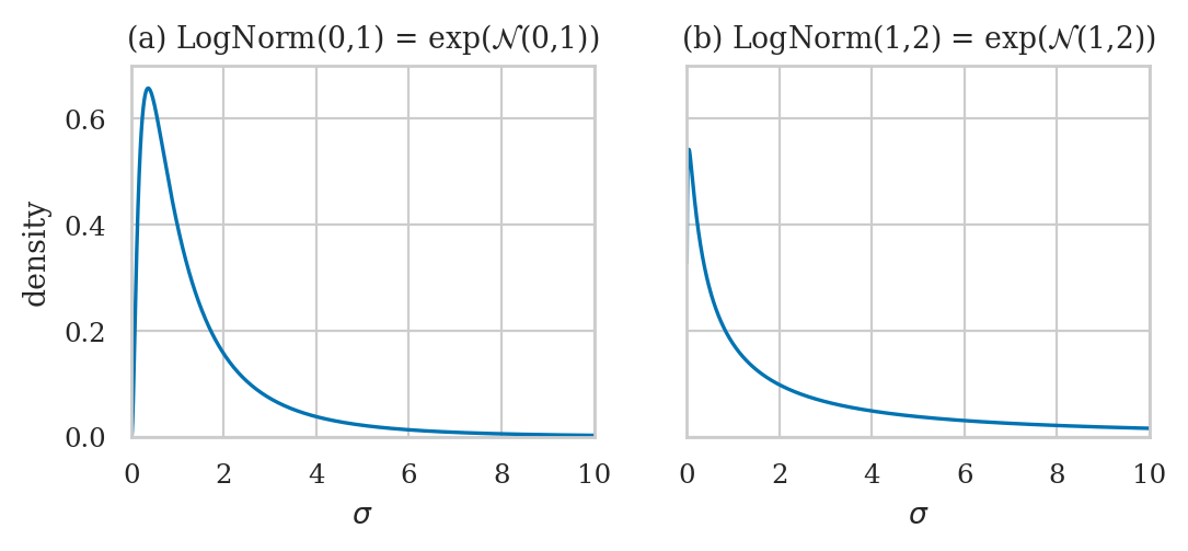
Choosing priors for log-sigma#

Normal distribution for log-sigma#

from scipy.stats import norm

def get_lognormal(mu=0, sigma=1):
    logsigs = np.linspace(-5, 5, 1000)
    dlogsigs = norm(mu, sigma).pdf(logsigs)
    sigmas = np.exp(logsigs)
    # Apply the change of variables to get the density for sigma
    # based on the Jacobian |d(log(sigma))/d(sigma)| = 1/sigma
    dsigmas = dlogsigs / sigmas
    return sigmas, dsigmas


with plt.rc_context({"figure.figsize":(6,2.2)}):
    fig, (ax1, ax2) = plt.subplots(1,2, sharey=True)

    # PLOT 1
    mu, sigma = 0, 1
    sigmas, dsigmas = get_lognormal(mu, sigma)
    sns.lineplot(x=sigmas, y=dsigmas, ax=ax1)
    ax1.set_xlabel('$\\sigma$')
    ax1.set_ylabel('density')
    ax1.set_title(f'(a) LogNorm({mu},{sigma}) = exp($\\mathcal{{N}}$({mu},{sigma}))')
    ax1.set_xlim(0, 10)
    ax1.set_ylim(0, 0.7)

    # PLOT 2
    mu, sigma = 1, 2
    sigmas, dsigmas = get_lognormal(mu, sigma)
    sns.lineplot(x=sigmas, y=dsigmas, ax=ax2)
    ax2.set_xlabel('$\\sigma$')
    ax2.set_ylabel('density')
    ax2.set_title(f'(b) LogNorm({mu},{sigma}) = exp($\\mathcal{{N}}$({mu},{sigma}))')
    ax2.set_xlim(0, 10)

../_images/775a576b5285b662853f64af2689c39811eddf6cdde49ff063f691a37df0eee4.png

Choosing priors for the degrees of freedom parameter#

# FIGURES ONLY
from scipy.stats import gamma
from scipy.stats import expon
from ministats import plot_pdf

with plt.rc_context({"figure.figsize":(6,2.2)}):
    fig, (ax1, ax2) = plt.subplots(1,2, sharey=True)

    # PLOT 1
    alpha, beta = 2, 0.1
    rv_nu = gamma(a=2, scale=1/beta)
    plot_pdf(rv_nu, rv_name="ν", ax=ax1)
    ax1.set_title(f'(a) Gamma($\\alpha=${alpha}, $\\beta=${beta})')
    ax1.set_xlim(0, 100)

    # PLOT 2
    scale = 30
    rv_nu_exp = expon(scale=scale)
    plot_pdf(rv_nu_exp, rv_name="ν", ax=ax2)
    ax2.set_title(f'(b) Expon($\\lambda=$1/{scale})')
    ax2.set_xlim(0, 100)

../_images/27690558c20f25f0c8f6397bfc46ae1aca65e2adfd8846ee241ccb16317e76bd.png

Example 1: comparing electricity prices#

Electricity prices from East End and West End

Electricity prices dataset#

eprices = pd.read_csv("../datasets/eprices.csv")
eprices.groupby("loc")["price"].describe()

	count	mean	std	min	25%	50%	75%	max
loc
East	9.0	6.155556	0.877655	4.8	5.5	6.3	6.5	7.7
West	9.0	9.155556	1.562139	6.8	8.3	8.6	10.0	11.8

eprices["price"].mean(), eprices["price"].std()

(7.655555555555556, 1.973120020267162)

Bayesian model#

\[\begin{align*} X_W \sim \mathcal{T}(\nu, M_W, \Sigma_W), \qquad \qquad X_E \sim \mathcal{T}(\nu, M_E, \Sigma_E), \qquad\qquad \\ M_W, M_E \!\sim\! \mathcal{N}(\mu_{M}, \sigma_{M}), \quad \log\Sigma_W, \log\Sigma_E\!\sim\!\mathcal{N}(0,1), \quad \nu \!\sim\! \text{Gamma}(2,0.1). \end{align*}\]

Bambi model#

formula1 = bmb.Formula("price ~ 0 + loc",
                       "sigma ~ 0 + loc")

links1 = {"mu":"identity",
          "sigma":"log"}

priors1 = {
    "loc": bmb.Prior("Normal", mu=8, sigma=5),
    "sigma": {
        "loc": bmb.Prior("Normal", mu=0, sigma=1)
    },
    "nu": bmb.Prior("Gamma", alpha=2, beta=0.1),
}

mod1 = bmb.Model(formula=formula1,
                 family="t",
                 link=links1,
                 priors=priors1,
                 data=eprices)
mod1

       Formula: price ~ 0 + loc
                sigma ~ 0 + loc
        Family: t
          Link: mu = identity
                sigma = log
  Observations: 18
        Priors: 
    target = mu
        Common-level effects
            loc ~ Normal(mu: 8.0, sigma: 5.0)
        
        Auxiliary parameters
            nu ~ Gamma(alpha: 2.0, beta: 0.1)
    target = sigma
        Common-level effects
            sigma_loc ~ Normal(mu: 0.0, sigma: 1.0)

mod1.build()
mod1.graph()

../_images/64dfbfc1e74c3b25292e4a71842e27350125f925d4286876ee45655832f8115d.svg

Prior predictive checks#

# TODO

Model fitting and analysis#

idata1 = mod1.fit(random_seed=42)

Initializing NUTS using jitter+adapt_diag...

/opt/hostedtoolcache/Python/3.10.17/x64/lib/python3.10/site-packages/pytensor/link/c/cmodule.py:2959: UserWarning: PyTensor could not link to a BLAS installation. Operations that might benefit from BLAS will be severely degraded.
This usually happens when PyTensor is installed via pip. We recommend it be installed via conda/mamba/pixi instead.
Alternatively, you can use an experimental backend such as Numba or JAX that perform their own BLAS optimizations, by setting `pytensor.config.mode == 'NUMBA'` or passing `mode='NUMBA'` when compiling a PyTensor function.
For more options and details see https://pytensor.readthedocs.io/en/latest/troubleshooting.html#how-do-i-configure-test-my-blas-library
  warnings.warn(

Multiprocess sampling (2 chains in 2 jobs)

NUTS: [nu, loc, sigma_loc]

Sampling 2 chains for 1_000 tune and 1_000 draw iterations (2_000 + 2_000 draws total) took 2 seconds.

We recommend running at least 4 chains for robust computation of convergence diagnostics

Processing the results#

Calculate derived quantities used for the analysis plots and summaries.

post1 = idata1["posterior"]

# Calculate sigmas from log-sigmas
#######################################################
logsig_W = post1["sigma_loc"].sel(sigma_loc_dim="West")
logsig_E = post1["sigma_loc"].sel(sigma_loc_dim="East")
post1["sigma_West"] = np.exp(logsig_W)
post1["sigma_East"] = np.exp(logsig_E)

# Calculate the difference between between means
post1["mu_West"] = post1["loc"].sel(loc_dim="West")
post1["mu_East"] = post1["loc"].sel(loc_dim="East")
post1["dmeans"] = post1["mu_West"] - post1["mu_East"]

# Calculate the difference between standard deviations
post1["dsigmas"] = post1["sigma_West"]-post1["sigma_East"]

# Effect size
#######################################################
pvar =(post1["sigma_West"]**2+post1["sigma_East"]**2)/2
post1["cohend"] = post1["dmeans"] / np.sqrt(pvar)

# #ALT: use helper function
# from ministats import calc_dmeans_stats
# calc_dmeans_stats(idata1, group_name="loc")

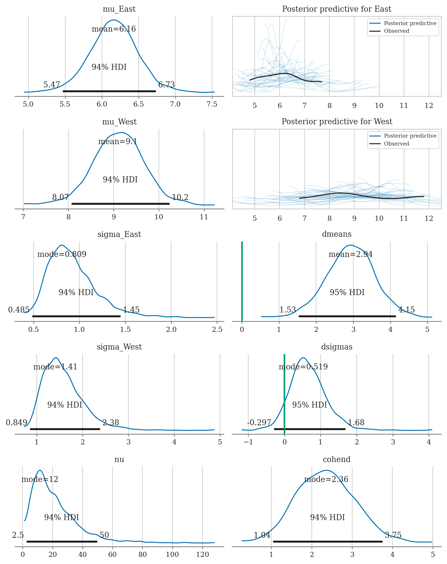
az.summary(idata1, kind="stats", hdi_prob=0.90,
           var_names=["mu_West", "mu_East", "dmeans", "sigma_West", "sigma_East", "dsigmas", "nu", "cohend"])

	mean	sd	hdi_5%	hdi_95%
mu_West	9.099	0.571	8.221	10.041
mu_East	6.163	0.333	5.616	6.681
dmeans	2.936	0.660	1.853	4.027
sigma_West	1.583	0.459	0.929	2.223
sigma_East	0.927	0.276	0.546	1.342
dsigmas	0.656	0.520	-0.183	1.440
nu	21.451	15.481	2.189	41.225
cohend	2.351	0.726	1.276	3.611

from ministats import plot_dmeans_stats
plot_dmeans_stats(mod1, idata1, group_name="loc");

../_images/aca551747f6aba033b490ac984244cf564b524ff247657dc78b26fcc06b3df22.png

Compare to frequentist results#

from scipy.stats import ttest_ind
pricesW = eprices[eprices["loc"]=="West"]["price"]
pricesE = eprices[eprices["loc"]=="East"]["price"]

res1 = ttest_ind(pricesW, pricesE, equal_var=False)
res1.statistic, res1.pvalue

(5.022875513276464, 0.0002570338337217609)

res1.confidence_interval(confidence_level=0.9)

ConfidenceInterval(low=1.9396575883681466, high=4.060342411631854)

from ministats import cohend2
cohend2(pricesW, pricesE)

2.3678062243290983

Conclusions#

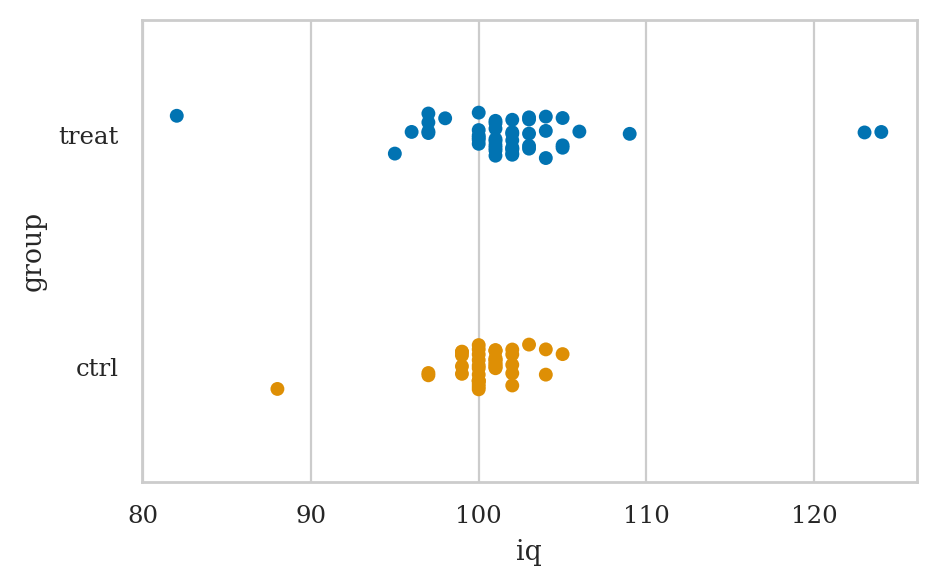
Example 2: comparing IQ scores#

We’ll look at IQ scores data taken from a the paper Bayesian Estimation Supersedes the t-Test (BEST) by John K. Kruschke.

smart drug administered to treatment group and want to compare to control group. Data contains outliers)

cf. compare_iqs2_many_ways.ipynb

IQ scores dataset#

iqs2 = pd.read_csv("../datasets/iqs2.csv")
iqs2.groupby("group")["iq"].describe()

	count	mean	std	min	25%	50%	75%	max
group
ctrl	42.0	100.357143	2.516496	88.0	100.0	100.5	101.0	105.0
treat	47.0	101.914894	6.021085	82.0	100.0	102.0	103.0	124.0

sns.stripplot(data=iqs2, x="iq", y="group", hue="group");

../_images/c1ab61972d30168dfeee2201386aa25de2dbaa3bccaa463b5ab4256cd136e78a.png

Bayesian model#

TODO: add formulas

Bambi model#

formula2 = bmb.Formula("iq ~ 0 + group",
                       "sigma ~ 0 + group")

priors2 = {
    "group": bmb.Prior("Normal", mu=100, sigma=35),
    "sigma": {
        "group": bmb.Prior("Normal", mu=1, sigma=2)
    },
    "nu": bmb.Prior("Gamma", alpha=2, beta=0.1),
}

mod2 = bmb.Model(formula=formula2,
                 family="t",
                 # link={"mu":"identity", "sigma":"log"}, # Bambi defaults
                 priors=priors2,
                 data=iqs2)

mod2

       Formula: iq ~ 0 + group
                sigma ~ 0 + group
        Family: t
          Link: mu = identity
                sigma = log
  Observations: 89
        Priors: 
    target = mu
        Common-level effects
            group ~ Normal(mu: 100.0, sigma: 35.0)
        
        Auxiliary parameters
            nu ~ Gamma(alpha: 2.0, beta: 0.1)
    target = sigma
        Common-level effects
            sigma_group ~ Normal(mu: 1.0, sigma: 2.0)

mod2.build()
mod2.graph()

../_images/457e432687be484cec7d804a2480c548b83954926ddb1d2bc783be0829225bb3.svg

Model fitting and analysis#

idata2 = mod2.fit(random_seed=42)

Initializing NUTS using jitter+adapt_diag...

Multiprocess sampling (2 chains in 2 jobs)

NUTS: [nu, group, sigma_group]

Sampling 2 chains for 1_000 tune and 1_000 draw iterations (2_000 + 2_000 draws total) took 2 seconds.

We recommend running at least 4 chains for robust computation of convergence diagnostics

from ministats import calc_dmeans_stats
calc_dmeans_stats(idata2, group_name="group");
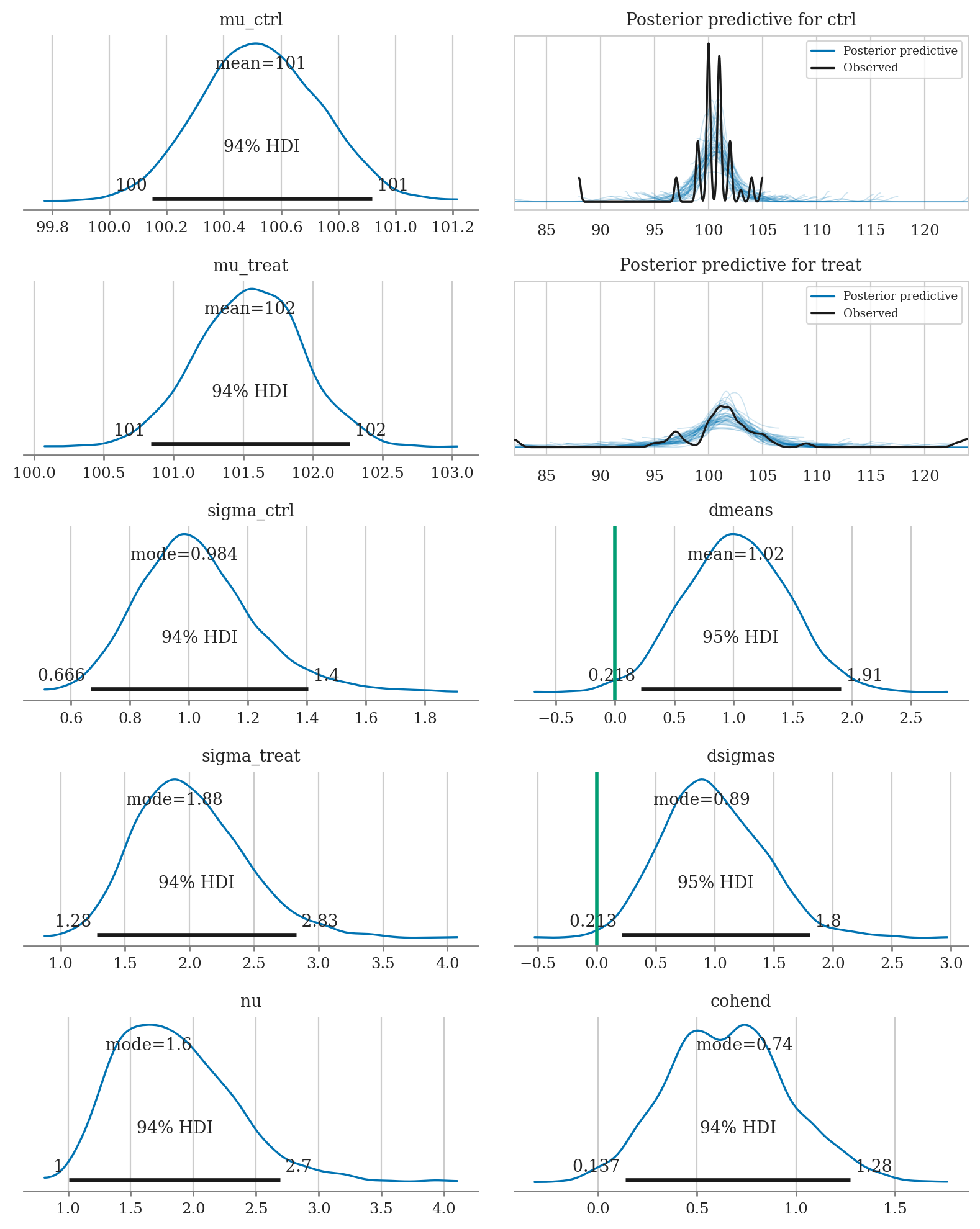
az.summary(idata2, kind="stats", hdi_prob=0.95,
           var_names=["mu_treat", "mu_ctrl", "dmeans", "sigma_treat", "sigma_ctrl", "dsigmas", "nu", "cohend"])

	mean	sd	hdi_2.5%	hdi_97.5%
mu_treat	101.547	0.379	100.807	102.285
mu_ctrl	100.528	0.209	100.150	100.947
dmeans	1.019	0.441	0.218	1.907
sigma_treat	2.006	0.422	1.228	2.839
sigma_ctrl	1.026	0.201	0.663	1.437
dsigmas	0.980	0.426	0.213	1.803
nu	1.859	0.487	1.002	2.773
cohend	0.660	0.307	0.091	1.291

from ministats import plot_dmeans_stats
plot_dmeans_stats(mod2, idata2, group_name="group", ppc_xlims=[82,124]);

../_images/66cac2fee1621e15ad88da444513e5c31e8b36547f2252561e5279b063572a5f.png

Sensitivity analysis#

from ministats.book.tables import sens_analysis_dmeans_iqs2
results = sens_analysis_dmeans_iqs2(iqs2)
results

---------------------------------------------------------------------------
ModuleNotFoundError                       Traceback (most recent call last)
Cell In[29], line 1
----> 1 from ministats.book.tables import sens_analysis_dmeans_iqs2
      2 results = sens_analysis_dmeans_iqs2(iqs2)
      3 results

ModuleNotFoundError: No module named 'ministats.book'

Compare to frequentist results#

from scipy.stats import ttest_ind

treated = iqs2[iqs2["group"]=="treat"]["iq"]
controls = iqs2[iqs2["group"]=="ctrl"]["iq"]

res2 = ttest_ind(treated, controls, equal_var=False)
res2.statistic, res2.pvalue

(1.622190457290228, 0.10975381983712836)

res2.confidence_interval(confidence_level=0.95)

ConfidenceInterval(low=-0.3611847716497789, high=3.476686291406612)

from ministats import cohend2
cohend2(treated, controls)

0.33096545301397307

# MAYBE
# # Test if the variances of the two groups are the same
# from scipy.stats import levene
# levene(treated, controls)

Conclusions#

Explanations#

Alternative choices of priors#

e.g. prior for sigma as very wiiiiiide, and nu ~ Exp(1/29)+1 → BEST Bayesian estimation supersedes the t-test by John K. Kruschke

If we use a model with common standard deviation, we get equivalent of pooled sigma

# TODO

Performance tests#

Simulated datasets#

Simulate datasets with various combinations of \(n\), \(\Delta\), and outliers.

from ministats.book.tables import gen_dmeans_datasets

ns = [20, 30, 50, 100]
Deltas = [0, 0.2, 0.5, 0.8, 1.3]
outliers_options = ["no", "few", "lots"]
dataset_specs = gen_dmeans_datasets(ns=ns,
                                    Deltas=Deltas,
                                    outliers_options=outliers_options)
dataset_specs[0:4]

[{'n': 20, 'Delta': 0, 'outliers': 'no', 'random_seed': 45},
 {'n': 20, 'Delta': 0, 'outliers': 'few', 'random_seed': 46},
 {'n': 20, 'Delta': 0, 'outliers': 'lots', 'random_seed': 47},
 {'n': 20, 'Delta': 0.2, 'outliers': 'no', 'random_seed': 48}]

Model comparisons#

Compare results several models:

Classical permutation test (from Section 4.5)
Classical Welch’s two-sample t-test (from Section 4.5)
Bayesian model with \(\mathcal{N}\) data model
Robust Bayesian model with \(\mathcal{T}\) data model
Bayes factors with JZS prior and standard cutoff

from ministats.book.tables import fit_dmeans_models
help(fit_dmeans_models)

Help on function fit_dmeans_models in module ministats.book.tables:

fit_dmeans_models(dataset, random_seed=42)
    Fit the following models for the difference of two means:
    - Permutation test from Section 3.5
    - Welch's two-sample $t$-test from Section 3.5
    - Bayesian model that uses normal as data model
    - Robust Bayesian model that uses t-distribution as data model
    - Bayes factor using JZS prior (using `pingouin` library)
    For each model, we run the hypothesis test to decide if the populations
    are the same or different based on the conventional cutoff level of 5%.
    We also construct a 90% confidnece interval for the diff. between `Delta`.

Results#

# Option A: load results from simulation
filename = "dmeans_perf_metrics__" \
            + "ns_20_30_50_100__" \
            + "Deltas_0_0.2_0.5_0.8_1.3__" \
            + "outs_no_few_lots__reps_100.csv"
results = pd.read_csv(os.path.join("simdata", filename), index_col=[0,1])
results.head(3)
# Option B: run full simulation (takes about three days)
# from ministats.book.tables import calc_dmeans_perf_metrics
# results = calc_dmeans_perf_metrics(reps=100)

		n	Delta	outliers	seed	count_reject	count_fail_to_reject	count_captured	avg_width
spec	model
0	perm	20	0.0	no	45	6	94	90.0	1.011714
	welch	20	0.0	no	45	6	94	90.0	1.065525
	norm_bayes	20	0.0	no	45	2	98	94.0	1.294730

Type I (false positive) error rates#

from ministats.book.tables import get_perf_table_typeI

tableA = get_perf_table_typeI(results)
tableA

	model	perm	welch	norm_bayes	robust_bayes	bf
outliers	n
no	20	0.06	0.06	0.02	0.07	0.02
	30	0.04	0.04	0.03	0.04	0.03
	50	0.04	0.04	0.01	0.04	0.01
	100	0.06	0.06	0.03	0.05	0.01
few	20	0.04	0.04	0.01	0.05	0.01
	30	0.04	0.04	0.01	0.05	0.00
	50	0.03	0.03	0.02	0.01	0.00
	100	0.07	0.07	0.06	0.08	0.03
lots	20	0.04	0.02	0.01	0.03	0.01
	30	0.02	0.02	0.00	0.02	0.00
	50	0.07	0.06	0.06	0.07	0.04
	100	0.03	0.03	0.03	0.02	0.00

Observations:

all models are about the same
BF model has significantly less false positives

Power analysis#

from ministats.book.tables import get_perf_table_power

tableB = get_perf_table_power(results, show_all=False)
tableB

		model	perm	welch	norm_bayes	robust_bayes	bf
outliers	Delta	n
no	0.5	30	0.46	0.46	0.33	0.46	0.31
		50	0.68	0.69	0.54	0.66	0.50
		100	0.93	0.93	0.90	0.93	0.84
	0.8	20	0.60	0.60	0.44	0.59	0.49
		30	0.86	0.86	0.77	0.86	0.72
		50	0.99	0.99	0.96	0.99	0.93
few	0.5	30	0.49	0.49	0.32	0.45	0.29
		50	0.49	0.51	0.39	0.58	0.33
		100	0.80	0.80	0.80	0.88	0.69
	0.8	20	0.69	0.68	0.51	0.65	0.54
		30	0.88	0.88	0.79	0.87	0.78
		50	0.85	0.85	0.83	0.94	0.75
lots	0.5	30	0.33	0.32	0.29	0.43	0.20
		50	0.52	0.52	0.50	0.63	0.33
		100	0.64	0.63	0.60	0.88	0.52
	0.8	20	0.44	0.43	0.37	0.63	0.30
		30	0.60	0.59	0.57	0.81	0.48
		50	0.82	0.83	0.79	0.97	0.66

Observations:

Bayes \(\mathcal{T}\) has higher power than Bayes \(\mathcal{N}\)
Bayes \(\mathcal{T}\) outperforms all other models when outliers are present

Interval estimates coverage#

from ministats.book.tables import get_perf_table_coverage

tableC = get_perf_table_coverage(results)
tableC

	model	perm		welch		norm_bayes		robust_bayes
		coverage	avg_width	coverage	avg_width	coverage	avg_width	coverage	avg_width
outliers	n
no	20	0.8800	1.011711	0.9050	1.064862	0.9650	1.298070	0.9100	1.078473
	30	0.9100	0.821001	0.9175	0.849298	0.9625	1.016220	0.9225	0.855460
	50	0.9050	0.651732	0.9100	0.665610	0.9525	0.762513	0.9100	0.667750
	100	0.9025	0.462228	0.9025	0.467091	0.9325	0.517568	0.9075	0.467747
few	20	0.8550	1.002797	0.8675	1.056252	0.9500	1.294572	0.8700	1.069132
	30	0.9175	0.835295	0.9250	0.864310	0.9625	1.022407	0.9250	0.872108
	50	0.8675	0.784709	0.9025	0.802027	0.9350	0.854340	0.9075	0.695260
	100	0.8725	0.554332	0.8975	0.560776	0.9125	0.581300	0.9275	0.487010
lots	20	0.8700	1.442238	0.9025	1.530370	0.9450	1.601472	0.8975	1.197020
	30	0.8550	1.085291	0.8700	1.128444	0.9000	1.197037	0.8550	0.926892
	50	0.8825	0.892523	0.8975	0.913113	0.9175	0.937645	0.9075	0.726270
	100	0.8975	0.679404	0.9025	0.686951	0.9175	0.688840	0.8950	0.509295

Observations:

All methods have coverage close to the nominal 90%
Bayes \(\mathcal{T}\) produces narrower intervals

Discussion#

Comparison to the frequentist two-sample t-test#

results numerically similar
note we’re using 𝒯 as data model, not as a sampling distribution
conceptually different:
- p-value vs. decision based on posterior distribution
- confidence intervals vs. credible intervals

Comparing multiple groups#

?Extension to Bayesian ANOVA? Can extend approach to multiple groups: Bayesian ANOVA

FWD reference to hierarchical models for group comparison covered in Section 5.5

Exercises#

Exercise 1: small samples#

As = [5.77, 5.33, 4.59, 4.33, 3.66, 4.48]
Bs = [3.88, 3.55, 3.29, 2.59, 2.33, 3.59]
groups = ["A"]*len(As) + ["B"]*len(Bs)
df1 = pd.DataFrame({"group": groups, "vals": As + Bs})
# df1

Exercise 2: lecture and debate curriculums#

students = pd.read_csv("../datasets/students.csv")
# students.groupby("curriculum")["score"].describe()

formula_std = bmb.Formula("score ~ 0 + curriculum",
                          "sigma ~ 0 + curriculum")
priors_std = {
    "curriculum": bmb.Prior("Normal", mu=70, sigma=30),
    "sigma": {
        "curriculum":bmb.Prior("Normal", mu=1, sigma=2)
    },
    "nu": bmb.Prior("Gamma", alpha=2, beta=0.1),
}
mod_std = bmb.Model(formula=formula_std,
                 family="t",
                 link="identity",
                 priors=priors_std,
                 data=students)
mod_std
# mod_std.build()
# mod_std.graph()

       Formula: score ~ 0 + curriculum
                sigma ~ 0 + curriculum
        Family: t
          Link: mu = identity
                sigma = log
  Observations: 15
        Priors: 
    target = mu
        Common-level effects
            curriculum ~ Normal(mu: 70.0, sigma: 30.0)
        
        Auxiliary parameters
            nu ~ Gamma(alpha: 2.0, beta: 0.1)
    target = sigma
        Common-level effects
            sigma_curriculum ~ Normal(mu: 1.0, sigma: 2.0)

idata_std = mod_std.fit(random_seed=42)

Initializing NUTS using jitter+adapt_diag...
Multiprocess sampling (4 chains in 4 jobs)
NUTS: [nu, curriculum, sigma_curriculum]

Sampling 4 chains for 1_000 tune and 1_000 draw iterations (4_000 + 4_000 draws total) took 3 seconds.

# Calculate the difference between between means
currs = idata_std["posterior"]["curriculum"]
mu_debate = currs.sel(curriculum_dim="debate")
mu_lecture = currs.sel(curriculum_dim="lecture")
idata_std["posterior"]["dmeans"] = mu_debate - mu_lecture
az.summary(idata_std, kind="stats", var_names=["dmeans"], hdi_prob=0.95)

	mean	sd	hdi_2.5%	hdi_97.5%
dmeans	7.61	5.301	-2.442	18.962

# from ministats import plot_dmeans_stats
# plot_dmeans_stats(mod_std, idata_std, ppc_xlims=[50,100], group_name="curriculum");

# from scipy.stats import ttest_ind
# scoresD = students[students["curriculum"]=="debate"]["score"]
# scoresL = students[students["curriculum"]=="lecture"]["score"]
# res_std = ttest_ind(scoresD, scoresL, equal_var=False)
# res_std.statistic, res_std.pvalue
# from ministats import cohend2
# cohend2(scoresL, scoresD)

Exercise 3: redo exercises from Section 3.5 section using Bayesian methods#

# TODO

Links#

TODO

BONUS Examples#

Example 4: small example form BEST vignette#

See http://cran.nexr.com/web/packages/BEST/vignettes/BEST.pdf#page=2

y1s = [5.77, 5.33, 4.59, 4.33, 3.66, 4.48]
y2s = [3.88, 3.55, 3.29, 2.59, 2.33, 3.59]

from ministats.bayes import bayes_dmeans
mod4, idata4 = bayes_dmeans(y1s, y2s, groups=["y1", "y2"])

Initializing NUTS using jitter+adapt_diag...
Multiprocess sampling (4 chains in 4 jobs)
NUTS: [nu, Intercept, group, sigma_group]

Sampling 4 chains for 1_000 tune and 2_000 draw iterations (4_000 + 8_000 draws total) took 2 seconds.

from ministats import calc_dmeans_stats
calc_dmeans_stats(idata4)
az.summary(idata4, kind="stats", hdi_prob=0.95,
           var_names=["dmeans", "sigma_y1", "sigma_y2", "dsigmas", "nu", "cohend"])

	mean	sd	hdi_2.5%	hdi_97.5%
dmeans	-1.436	0.501	-2.400	-0.413
sigma_y1	0.861	0.332	0.368	1.522
sigma_y2	0.717	0.287	0.305	1.246
dsigmas	-0.144	0.439	-1.016	0.726
nu	21.408	13.799	1.488	48.269
cohend	-1.900	0.780	-3.462	-0.425

# from ministats import plot_dmeans_stats
# plot_dmeans_stats(mod4, idata4, ppc_xlims=None);

Example 5: comparing morning to evening#

treszkai/best

morning = [8.99, 9.21, 9.03, 9.15, 8.68, 8.82, 8.66, 8.82, 8.59, 8.14,
           9.09, 8.80, 8.18, 9.23, 8.55, 9.03, 9.36, 9.06, 9.57, 8.38]
evening = [9.82, 9.34, 9.73, 9.93, 9.33, 9.41, 9.48, 9.14, 8.62, 8.60,
           9.60, 9.41, 8.43, 9.77, 8.96, 9.81, 9.75, 9.50, 9.90, 9.13]

from ministats.bayes import bayes_dmeans
mod5, idata5 = bayes_dmeans(evening, morning, groups=["evening", "morning"])

Initializing NUTS using jitter+adapt_diag...
Multiprocess sampling (4 chains in 4 jobs)
NUTS: [nu, Intercept, group, sigma_group]

Sampling 4 chains for 1_000 tune and 2_000 draw iterations (4_000 + 8_000 draws total) took 5 seconds.

from ministats import calc_dmeans_stats
calc_dmeans_stats(idata5)
az.summary(idata5, kind="stats", hdi_prob=0.95,
           var_names=["dmeans", "sigma_evening", "sigma_morning", "dsigmas", "nu", "cohend"])

	mean	sd	hdi_2.5%	hdi_97.5%
dmeans	-0.527	0.141	-0.803	-0.250
sigma_evening	0.454	0.085	0.303	0.627
sigma_morning	0.387	0.072	0.257	0.531
dsigmas	-0.067	0.109	-0.276	0.157
nu	23.126	14.430	3.036	51.899
cohend	-1.265	0.383	-2.011	-0.508

# from ministats import plot_dmeans_stats
# plot_dmeans_stats(mod5, idata5, ppc_xlims=None);

Section 5.4 — Bayesian difference between means

Contents

Section 5.4 — Bayesian difference between means#

Notebook setup#

Introduciton#

Model#

Bambi formula objects#

Choosing priors for log-sigma#

Normal distribution for log-sigma#

Choosing priors for the degrees of freedom parameter#

Example 1: comparing electricity prices#

Electricity prices dataset#

Bayesian model#

Bambi model#

Prior predictive checks#

Model fitting and analysis#

Processing the results#

Compare to frequentist results#

Conclusions#

Example 2: comparing IQ scores#

IQ scores dataset#

Bayesian model#

Bambi model#

Model fitting and analysis#

Sensitivity analysis#

Compare to frequentist results#

Conclusions#

Explanations#

Alternative choices of priors#

Performance tests#

Simulated datasets#

Model comparisons#

Results#

Type I (false positive) error rates#

Power analysis#

Interval estimates coverage#

Discussion#

Comparison to the frequentist two-sample t-test#

Comparing multiple groups#

Exercises#

Exercise 1: small samples#

Exercise 2: lecture and debate curriculums#

Exercise 3: redo exercises from Section 3.5 section using Bayesian methods#

Links#

BONUS Examples#

Example 4: small example form BEST vignette#

Example 5: comparing morning to evening#