Section 2.5 — Continuous random variables#
This notebook contains all the code examples from Section 2.5 Continuous random variables of the No Bullshit Guide to Statistics.
Topics covered in this notebook:
Definitions of continuous random variables
Examples of random variables
Probability calculations
Computer models for random variables
Overview of
scipy.statsmethods
Real-world example to demo probability applications
Discussion
Bulk and tails of a the normal distribution
Notebook setup#
We’ll start by importing the Python modules we’ll need for this notebook.
# load Python modules
import numpy as np
import pandas as pd
import seaborn as sns
import matplotlib.pyplot as plt
# Figures setup
sns.set_theme(
    context="paper",
    style="whitegrid",
    palette="colorblind",
    rc={'figure.figsize': (7,2)},
)
%config InlineBackend.figure_format = 'retina'
%pip install -q ministats
Note: you may need to restart the kernel to use updated packages.
from ministats import plot_pdf_and_cdf
# set random seed for repeatability
np.random.seed(3)
Definitions#
Random variables#
random variable \(X\): a quantity that can take on different values.
outcome: a particular value \(\{X = x\}\) or range of values \(\{a \leq X \leq b\}\) that can occur as a result of observing the random variable \(X\).
sample space \(\mathcal{X}\): describes the set of all possible outcomes of the random variable.
\(f_X\): the probability distribution function is a function that assigns probabilities to the different outcome in the sample space of a random variable. The probability distribution function of the random variable \(X\) is a function of the form \(f_X: \mathcal{X} \to \mathbb{R}\).
\(F_X\): the cumulative distribution function (CDF) tells us the probability of an outcome less than or equal to a given value: \(F_X(b) = Pr(\{ X \leq b \})\).
\(F_X^{-1}\): the inverse cumulative distribution function computes contains the information about the quantiles of the probability distribution. The value \(F_X^{-1}(q)=x_q\) tells how far you need to go in the sample space so that the event \(\{ X \leq x_q \}\) contains a proportion \(q\) of the total probability: \(\Pr(\{ X \leq x_q \})=q\).
\(\mathbb{E}_X[w]\): the expected value of the function \(w(X)\) computes the average value of \(w(X)\) computed for all the possible values of the random variable \(X\).
Example 1: Uniform distribution#
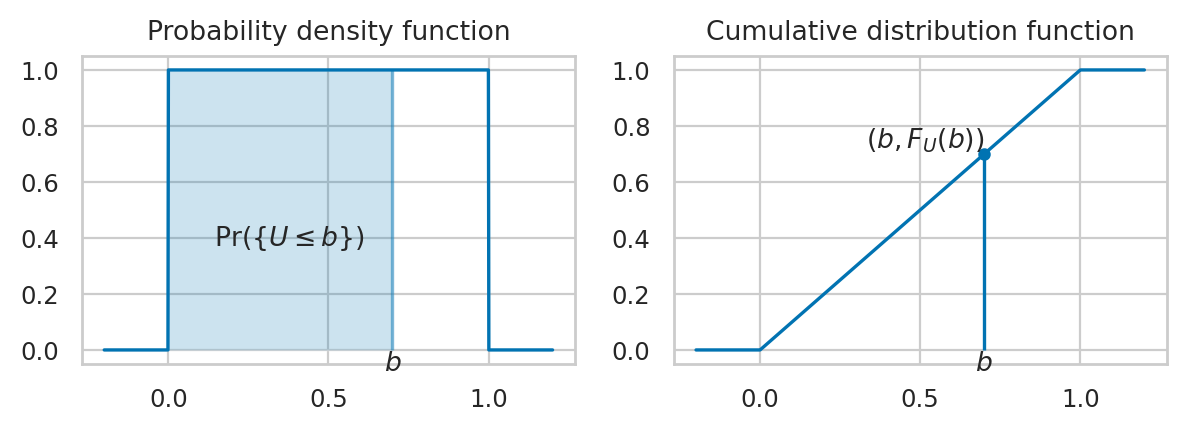
The uniform distribution \(\mathcal{U}(0,1)\) is described by the following probability density function:
where \(U\) is the name of the random variable and \(u\) are particular values it can take on.
The above equation describes tells you how likely it is to observe \(\{U=u\}\). For a uniform distribution \(\mathcal{U}(0,1)\), each \(u\) between 0 and 1 is equally likely to occur, and values of \(u\) outside this range have zero probability of occurring.
Computer simulation
The continuous uniform family of distribution \(\mathcal{U}(\alpha,\beta)\), which assigns equal probabilities to all outcomes in the interval \([\alpha,\beta]\). To create a computer model for a continuous uniform distribution, use the code
uniform(alpha,beta), wherealphaandbetaare two floats.
We’ll introduce computer models for random variables is Section 2.1.5 — Computer models for random variables below, but since we’re looking at a notebook, we can show a little preview of the calculations you’ll learn by the end of the section.
# define the computer model `rvU` for the random variable U
from scipy.stats import uniform
rvU = uniform(0, 1)

# use `quad` function to integrate rvU.pdf between 0.2 and 0.5
from scipy.integrate import quad
quad(rvU.pdf, 0.2, 0.5)[0]
0.3
plot_pdf_and_cdf(rvU, b=0.7, xlims=[-0.2,1.2], rv_name="U");
Example 2: Normal distribution#
A random variable \(N\) with a normal distribution \(\mathcal{N}(\mu,\sigma)\) is described by the probability density function:
The mean \(\mu\) (the Greek letter mu) and the standard deviation \(\sigma\) (the Greek letter sigma) are called the parameters of the distribution.
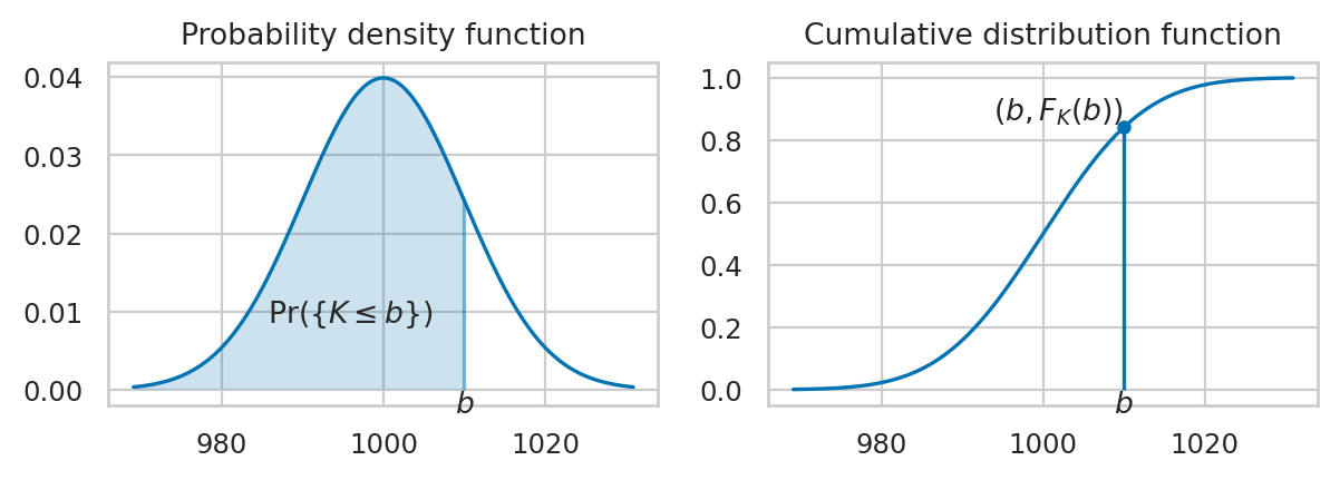
The math notation \(\mathcal{N}(\mu, \sigma)\) is used to describe the whole family of normal probability distributions, and \(K \sim \mathcal{N}(\mu_K=1000, \sigma_K=10)\) is a particular instance of the distribution with mean \(\mu_K = 1000\) and standard deviation \(\sigma_K = 10\).
The code example below shows the calculation of the probability \(\Pr\!\left( \{ 980 \leq K \leq 990 \} \right)\), which corresponds to the integral \(\int_{k=980}^{k=990} f_K(k) dk\).
# define the computer model `rvK` for the random variable K
from scipy.stats import norm
muK = 1000
sigmaK = 10
rvK = norm(muK, sigmaK)

# use `quad` function to integrate rvK.pdf between 980 and 990
quad(rvK.pdf, 980, 990)[0]
0.13590512198327784
plot_pdf_and_cdf(rvK, b=1010, rv_name="K");
Calculations with random variables#
Example 1: mean and variance of the uniform distribution#
Mean#
# from sympy import symbols, integrate
# u = symbols('u')
# integrate(u * 1, (u,0,1))
from scipy.integrate import quad

def u_times_fU(u):
	return u * 1

quad(u_times_fU, 0, 1)[0]
0.5
So the mean is \(\mu_U = \frac{1}{2} = 0.5\).
Variance#
The formula for the variance is
# from sympy import symbols, integrate
# u = symbols('u')
# integrate( (u-1/2)**2 * 1, (u,0,1) )
def u_minus_muU_squared(u):
    return (u-0.5)**2

quad(u_minus_muU_squared, 0, 1)[0]
0.08333333333333333
So the variance of \(U\) is \(\sigma_U^2 = 0.08\overline{3} = \frac{1}{12}\).
We can compute the standard deviation \(\sigma_U\) by taking the square root of the variance.
import numpy as np
np.sqrt(0.0833333333333333)
0.2886751345948128
Example 2: mean and variance of a normal distribution#
import numpy as np

muK = 1000
sigmaK = 10

def fK(k):
    z = (k - muK) / sigmaK
    C = sigmaK * np.sqrt(2*np.pi)
    return 1 / C * np.exp(-1/2 * z**2)
The mean of \(K\) is
from scipy.integrate import quad

def k_times_fK(k):
    return k * fK(k)

quad(k_times_fK, 0, 2000)[0]
999.9999999999997
The standard deviation of \(K\) is
def k_minus_meanK_sq_times_fK(k):
    return (k - 1000)**2 * fK(k)

quad(k_minus_meanK_sq_times_fK, 0, 2000)[0]
100.00000000000006
Skewness and kurtosis#
rvK.stats("s")
0.0
rvK.stats("k")
0.0
Computer models for random variables#
<model>: the family of probability distributions<params>: parameters of the model—specific value of the control knobs we choose in the general family of distributions to create a particular distribution<model>(<params>): a particular instance of probability model created by choosing a model family<model>and the model parameters<params>.example 1: uniform family of distribution \(\mathcal{U}(\alpha,\beta)\) with parameters \(\alpha\) and \(\beta\).
example 2: normal family of distribution \(\mathcal{N}(\mu,\sigma)\) with parameters \(\mu\) and \(\sigma\).
\(\sim\): math shorthand symbol that stands for “is distributed according to.” For example \(X \sim \texttt{model}(\theta)\) means the random variable \(X\) is distributed according to model instance \(\texttt{model}\) and parameters \(\theta\).
from scipy.stats import norm

# create a normal random variable with mean 1000 and std 10
rvK = norm(1000, 10)
type(rvK)
scipy.stats._distn_infrastructure.rv_continuous_frozen
## see all attributes and methods:
# [attr for attr in dir(rvK) if "__" not in attr]
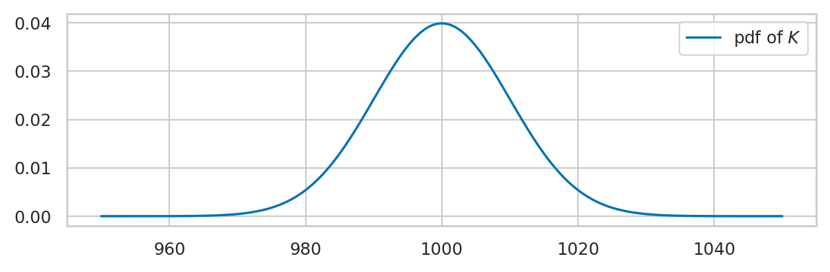
Plotting the probability density function#
ks = np.linspace(950, 1050, 1000)
fKs = rvK.pdf(ks)
sns.lineplot(x=ks, y=fKs, label="pdf of $K$");
The cumulative distribution is the integral of the probability density function:
ks = np.linspace(950, 1050, 1000)
FKs = rvK.cdf(ks)
sns.lineplot(x=ks, y=FKs, label="CDF of $K$");

Properties of the distribution#
rvK.mean()
1000.0
rvK.std()
10.0
rvK.var()
100.0
rvK.std() # == np.sqrt(rvK.var())
10.0
rvK.median()
1000.0
rvK.support()
(-inf, inf)
Computing probabilities#
Suppose you want to compute the probability of the outcome \(\{ a \leq K \leq b \}\) for the random variable \(K\).
# Pr({980 < N < 1020}) = integral of f_N between 980 and 1020
quad(rvK.pdf, 980, 1020)[0]
0.9544997361036411
# Pr({980 < N < 1020}) = F_N(1020) - F_N(980)
rvK.cdf(1020) - rvK.cdf(980)
0.9544997361036416
Computing quantiles#
The inverse question is to find the interval \((-\infty, k_q]\) that contains proportion \(q\) of the total probability.
First quartile#
The first quartile (\(q=0.25\) quantile) is located at \(F_K^{-1}(0.25)\)
rvK.ppf(0.25)
993.2551024980392
We can verify that \(\Pr({K \leq 993.2551024980392)}) = 0.25\)
rvK.cdf(993.2551024980392)
0.24999999999999895
Second quartile#
rvK.ppf(0.5)
1000.0
Third quartile#
rvK.ppf(0.75)
1006.7448975019608
Left tail#
rvK.ppf(0.05)
983.5514637304852
Right tail#
rvK.ppf(0.95)
1016.4485362695148
Computing confidence intervals#
To compute a 90% confidence interval for the random variable \(K\),
we can call the rvK.ppf() twice.
[rvK.ppf(0.05), rvK.ppf(0.95)]
[983.5514637304852, 1016.4485362695148]
Generating random observations#
Let’s say you want to generate \(n=10\) observations from the random variable \(N\).
You can do this by calling the method rvN.rvs(n).
np.random.seed(45)

ksample = rvK.rvs(10)
ksample.round(2)
array([1000.26, 1002.6 ,  996.05,  997.96,  987.28,  974.03, 1002.9 ,
        991.27, 1003.94, 1009.35])
Sample mean#
np.mean(ksample)
996.5642932112244
Sample standard deviation#
np.std(ksample, ddof=1)
10.177891977273164
Computing expectations#
Suppose the distributor accepts only bottles contain between 980 ml and 1020 ml, and you’ll receive a receive payment of \(\$2\) for each bottle. Bottles outside that range get rejected and you don’t get paid for them.
def payment(k):
    if 980 <= k and k <= 1020:
        return 2
    else:
        return 0
# get paid if in spec
payment(1005)
2
# don't get paid if out of spec
payment(1025)
0
# expected value of payment
rvK.expect(payment, lb=0, ub=2000)
1.9089994711961735
Visually speaking, only parts of the probability mass of the random variable “count” towards the payment, the subset of the values inside the yellow region shown below.
ks = np.linspace(900, 1100, 1000)
payments = [payment(k)/50 for k in ks]

sns.lineplot(x=ks, y=rvK.pdf(ks))
sns.lineplot(x=ks, y=payments, label="payment(k)")
<Axes: >

Multiple random variables#
Joint probability density functions#
TODO: insert figure as attachment here.
See notebook ../figure_generation/continuous_RVs.ipynb for the code to generate the figure in the book.
Marginal density functions#
TODO: insert figure as attachment here.
See notebook ../figure_generation/continuous_RVs.ipynb for the code to generate the figure in the book.
Conditional probability density functions#
Examples#
Example ?: Multivariate normal#
# TODO
Useful probability formulas#
Multivariable expectation#
Independent, identically distributed random variabls#
Discussion#
Bulk of the normal distribution#
How much of the total probability “weight” lies within \(n\) standard deviations of the mean?
from scipy.stats import norm
rvK = norm(1000, 10)
from scipy.integrate import quad

muK = rvK.mean()    # mean of the random variable rvK
sigmaK = rvK.std()  # standard deviation of rvK

for n in [1, 2, 3]:
    I_n = [muK - n*sigmaK, muK + n*sigmaK]
    p_n = quad(rvK.pdf, I_n[0], I_n[1])[0]
    print(f"p_{n} = Pr( K in {I_n} ) = {p_n:.3f}")
p_1 = Pr( K in [990.0, 1010.0] ) = 0.683
p_2 = Pr( K in [980.0, 1020.0] ) = 0.954
p_3 = Pr( K in [970.0, 1030.0] ) = 0.997
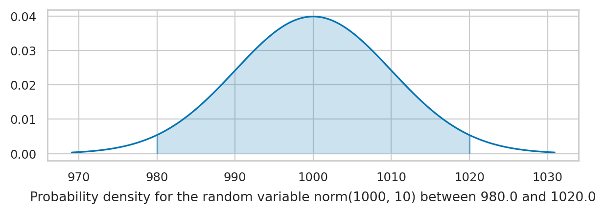
The code below highlights the interval \(I_n\) and computes the probability \(p_n\).
Change the value of the variable n to get different plots.
from ministats import calc_prob_and_plot

n = 2  # number of standard deviations around the mean

# values of x in the interval 𝜇 ± n𝜎 = [𝜇-n𝜎, 𝜇+n𝜎]
I_n = [muK - n*sigmaK, muK + n*sigmaK]
p_n, _ = calc_prob_and_plot(rvK, I_n[0], I_n[1])
p_n
0.9544997361036411
Try changing the value of the variable n to 1 or 3 in the above code cell.
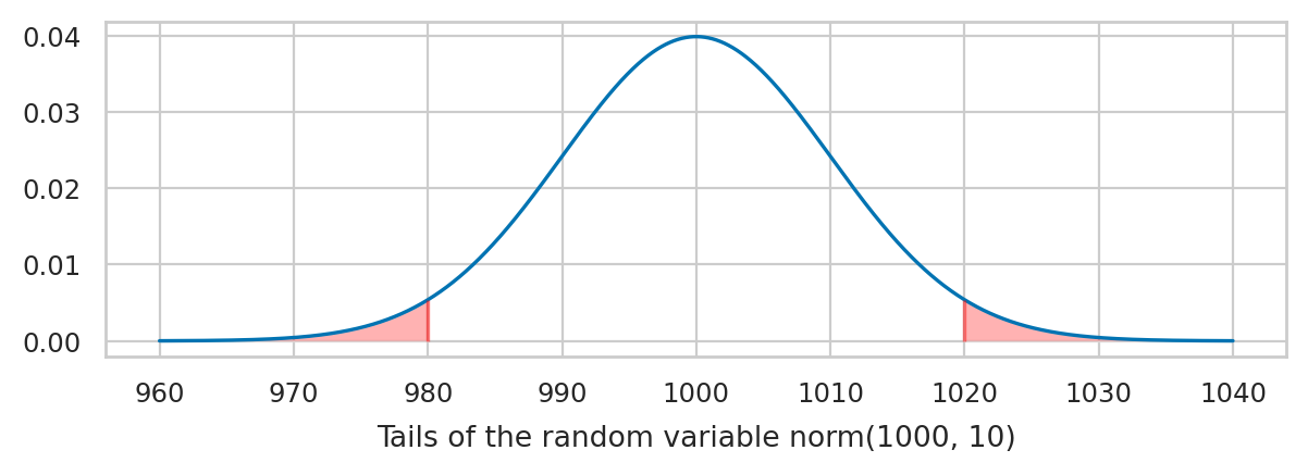
Tails of the normal distribution#
We’re often interested in tail ends of the distribution, which contain the unlikely events.
muK = rvK.mean()    # mean of the random variable rvK
sigmaK = rvK.std()  # standard deviation of rvK

for n in [1, 2, 3]:
    # compute the probability in the left tail (-∞,𝜇-n𝜎]
    x_l = muK - n*sigmaK
    p_l = quad(rvK.pdf, rvK.ppf(0.0000000001), x_l)[0]
    # compute the probability in the right tail [𝜇+n𝜎,∞)
    x_r = muK + n*sigmaK
    p_r = quad(rvK.pdf, x_r, rvK.ppf(0.9999999999))[0]
    # add together to get total probability in the tails
    p_tails = p_l + p_r
    print(f"Pr( K<{x_l} or K>{x_r} ) = {p_tails:.4f}")
Pr( K<990.0 or K>1010.0 ) = 0.3173
Pr( K<980.0 or K>1020.0 ) = 0.0455
Pr( K<970.0 or K>1030.0 ) = 0.0027
The code below highlights the tails of the distribution and computes the sum of their probability.
from ministats import calc_prob_and_plot_tails

muK = rvK.mean()    # mean of the random variable rvK
sigmaK = rvK.std()  # standard deviation of rvK

n = 2  # number of standard deviations around the mean

# the distribution's left tail (-∞,𝜇-k𝜎]
x_l = muK - n*sigmaK
# the distribution's right tail [𝜇+k𝜎,∞)
x_r = muK + n*sigmaK
p_tails, _ = calc_prob_and_plot_tails(rvK, x_l, x_r, xlims=[960, 1040])

print(f"Pr( {{K<{x_l}}} ∪ {{K>{x_r}}} ) = {p_tails:.4f}")
Pr( {K<980.0} ∪ {K>1020.0} ) = 0.0455
Try changing the value of the variable k in the above code cell.
The above calculations leads us to an important rule of thumb: the values of the 5% tail of the distribution are \(n=2\) standard deviations away from the mean (more precisely, we should use \(n=1.96\) to get exactly 5%). We’ll use this facts later in STATS to define a cutoff value for events that are unlikely to occur by chance.