Section 5.2 — Bayesian inference computations

Section 5.2 — Bayesian inference computations#

This notebook contains the code examples from Section 5.2 Bayesian inference computations from the No Bullshit Guide to Statistics.

Notebook setup#

# load Python modules
import os
import numpy as np
import pandas as pd
import seaborn as sns
import matplotlib.pyplot as plt

# Figures setup
plt.clf()  # needed otherwise `sns.set_theme` doesn"t work
from plot_helpers import RCPARAMS
RCPARAMS.update({"figure.figsize": (5, 3)})   # good for screen
# RCPARAMS.update({"figure.figsize": (5, 2)})  # good for print
sns.set_theme(
    context="paper",
    style="whitegrid",
    palette="colorblind",
    rc=RCPARAMS,
)

# High-resolution please
%config InlineBackend.figure_format = "retina"

#######################################################

<Figure size 640x480 with 0 Axes>

Definitions#

TODO

Posterior inference using MCMC estimation#

TODO: point-form definitions

Bayesian inference using Bambi#

TODO: mention Bambi classes

import bambi as bmb

print(bmb.Prior.__doc__)

Abstract specification of a term prior

    Parameters
    ----------
    name : str
        Name of prior distribution. Must be the name of a PyMC distribution
        (e.g., `"Normal"`, `"Bernoulli"`, etc.)
    auto_scale: bool
        Whether to adjust the parameters of the prior or use them as passed. Default to `True`.
    kwargs : dict
        Optional keywords specifying the parameters of the named distribution.
    dist : pymc.distributions.distribution.DistributionMeta or callable
        A callable that returns a valid PyMC distribution. The signature must contain `name`,
        `dims`, and `shape`, as well as its own keyworded arguments.
    

print("\n".join(bmb.Model.__doc__.splitlines()[0:27]))

Specification of model class

    Parameters
    ----------
    formula : str or bambi.formula.Formula
        A model description written using the formula syntax from the `formulae` library.
    data : pandas.DataFrame
        A pandas dataframe containing the data on which the model will be fit, with column
        names matching variables defined in the formula.
    family : str or bambi.families.Family
        A specification of the model family (analogous to the family object in R). Either
        a string, or an instance of class `bambi.families.Family`. If a string is passed, a
        family with the corresponding name must be defined in the defaults loaded at `Model`
        initialization. Valid pre-defined families are `"bernoulli"`, `"beta"`,
        `"binomial"`, `"categorical"`, `"gamma"`, `"gaussian"`, `"negativebinomial"`,
        `"poisson"`, `"t"`, and `"wald"`. Defaults to `"gaussian"`.
    priors : dict
        Optional specification of priors for one or more terms. A dictionary where the keys are
        the names of terms in the model, "common," or "group_specific" and the values are
        instances of class `Prior`. If priors are unset, uses automatic priors inspired by
        the R rstanarm library.
    link : str or Dict[str, str]
        The name of the link function to use. Valid names are `"cloglog"`, `"identity"`,
        `"inverse_squared"`, `"inverse"`, `"log"`, `"logit"`, `"probit"`, and
        `"softmax"`. Not all the link functions can be used with all the families.
        If a dictionary, keys are the names of the target parameters and the values are the names
        of the link functions.

Example 1: estimating the probability of a bias of a coin#

Let’s revisit the biased coin example from Section 5.1, where we want to estimate the probability the coin turns up heads.

Data#

We have a sample that contains \(n=50\) observations (coin tosses) from the coin. The outcome 1 corresponds to heads, while the outcome 0 corresponds to tails. We package the data as the ctoss column of a new data frame ctosses.

ctosses = [1,1,0,0,1,0,1,1,1,1,1,0,1,1,0,0,0,1,1,1,
           1,1,1,1,1,1,1,0,1,1,1,1,1,1,1,1,0,0,1,0,
           0,1,0,1,0,1,0,1,1,0]
ctosses = pd.DataFrame({"ctoss":ctosses})
ctosses.head(3)

	ctoss
0	1
1	1
2	0

The proportion of heads outcomes is:

ctosses["ctoss"].mean()

0.68

Model#

The model is

\[ C \sim \textrm{Bernoulli}(P), \qquad P \sim \mathcal{U}(0,1). \]

import bambi as bmb
bmb.Prior("Uniform", lower=0, upper=1)

Uniform(lower: 0.0, upper: 1.0)

priors1 = {
    "Intercept": bmb.Prior("Uniform", lower=0, upper=1)
}

mod1 = bmb.Model(formula="ctoss ~ 1",
                 family="bernoulli",
                 link="identity",
                 priors=priors1,
                 data=ctosses)
mod1.set_alias({"Intercept": "P"})
mod1

       Formula: ctoss ~ 1
        Family: bernoulli
          Link: p = identity
  Observations: 50
        Priors: 
    target = p
        Common-level effects
            Intercept ~ Uniform(lower: 0.0, upper: 1.0)

mod1.build()
mod1.graph()

../_images/1dbded6b943a483e1c3253c0be6e0a735258ca2698ad8d827c4637b594e73855.svg

# mod1.backend.model

Fitting the model#

idata1 = mod1.fit(random_seed=42)

Modeling the probability that ctoss==1

Initializing NUTS using jitter+adapt_diag...

Multiprocess sampling (2 chains in 2 jobs)

NUTS: [P]

Sampling 2 chains for 1_000 tune and 1_000 draw iterations (2_000 + 2_000 draws total) took 1 seconds.

We recommend running at least 4 chains for robust computation of convergence diagnostics

Extracting the samples from the posterior#

postP = idata1["posterior"]["P"].values.flatten()
postP

array([0.76122756, 0.56861221, 0.77616961, ..., 0.60182373, 0.59438488,
       0.6632119 ])

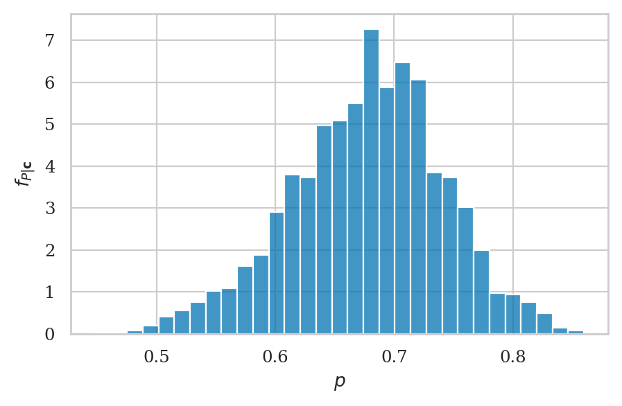
Visualize the posterior#

Histogram#

ax = sns.histplot(x=postP, stat="density")
ax.set_xlabel("$p$")
ax.set_ylabel("$f_{P|\\mathbf{c}}$");

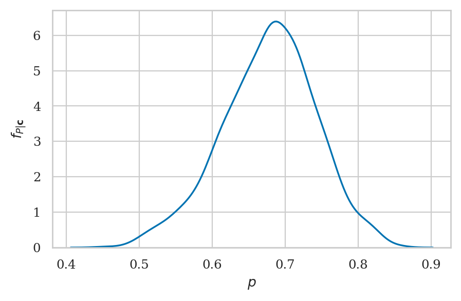
../_images/82a8b46bf4e8c6c6489dac866d2f69599b675ac536f2a24d5a405014e5745ec9.png

Kernel density plot#

ax = sns.kdeplot(x=postP)
ax.set_xlabel("$p$")
ax.set_ylabel("$f_{P|\\mathbf{c}}$");

../_images/459c16f191bebf7e63fdbd037e46d3a7655ea64fa890f9c1c62e5063e6f87024.png

Summarize the posterior#

len(postP)

Posterior mean#

np.mean(postP)

0.6774457022266422

Posterior standard deviation#

np.std(postP)

0.06465710325405617

Posterior median#

np.median(postP)

0.6816845607499968

Posterior quartiles#

np.quantile(postP, [0.25, 0.5, 0.75])

array([0.63596093, 0.68168456, 0.72070423])

Posterior percentiles#

np.percentile(postP, [3, 97])

array([0.54584942, 0.79597242])

Posterior mode#

from ministats import mode_from_samples
mode_from_samples(postP)

0.6872105271863933

Credible interval#

from ministats import hdi_from_samples
hdi_from_samples(postP, hdi_prob=0.9)

[0.5677606764344124, 0.7802343628275518]

Example 2: estimating the IQ score#

Let’s return to the investigation of the smart drug effects on IQ scores.

Data#

We have collected data from \(30\) individuals who took the smart drug, which we have packaged into the iq column of the data frame iqs.

iqs = [ 82.6, 105.5,  96.7,  84.0, 127.2,  98.8,  94.3,
       122.1,  86.8,  86.1, 107.9, 118.9, 116.5, 101.0,
        91.0, 130.0, 155.7, 120.8, 107.9, 117.1, 100.1,
       108.2,  99.8, 103.6, 108.1, 110.3, 101.8, 131.7,
       103.8, 116.4]
iqs = pd.DataFrame({"iq":iqs})
iqs["iq"].mean()

107.82333333333334

Model#

We will use the following Bayesian model:

\[ X \sim \mathcal{N}(M, \sigma=15), \qquad M \sim \mathcal{N}(\mu_M=100,\sigma_M=40). \]

We place a broad prior on the mean parameter \(M\), by choosing a large value for the standard deviation \(\sigma_M\). We assume the IQ scores come from a population with standard deviation \(\sigma = 15\).

import bambi as bmb

priors2 = {
    "Intercept": bmb.Prior("Normal", mu=100, sigma=40),
    "sigma": 15,
}

mod2 = bmb.Model(formula="iq ~ 1",
                 family="gaussian",
                 link="identity",
                 priors=priors2,
                 data=iqs)

mod2.set_alias({"Intercept": "M"})
mod2

       Formula: iq ~ 1
        Family: gaussian
          Link: mu = identity
  Observations: 30
        Priors: 
    target = mu
        Common-level effects
            Intercept ~ Normal(mu: 100.0, sigma: 40.0)
        
        Auxiliary parameters
            sigma ~ 15

mod2.build()
mod2.graph()

../_images/1eaacde2e9af6fcf79211f744a4dc47ef562318025b01ac5e5f949edf931cbd7.svg

Fitting the model#

This time we’ll generate \(N=2000\) samples from each chain.

idata2 = mod2.fit(draws=2000, random_seed=42)

Initializing NUTS using jitter+adapt_diag...

Multiprocess sampling (2 chains in 2 jobs)

NUTS: [M]

Sampling 2 chains for 1_000 tune and 2_000 draw iterations (2_000 + 4_000 draws total) took 1 seconds.

We recommend running at least 4 chains for robust computation of convergence diagnostics

Extract the samples from the posterior#

postM = idata2["posterior"]["M"].values.flatten()
len(postM)

postM

array([111.84188777, 111.84188777, 110.69558723, ..., 107.81737867,
       110.06495156, 108.77654813])

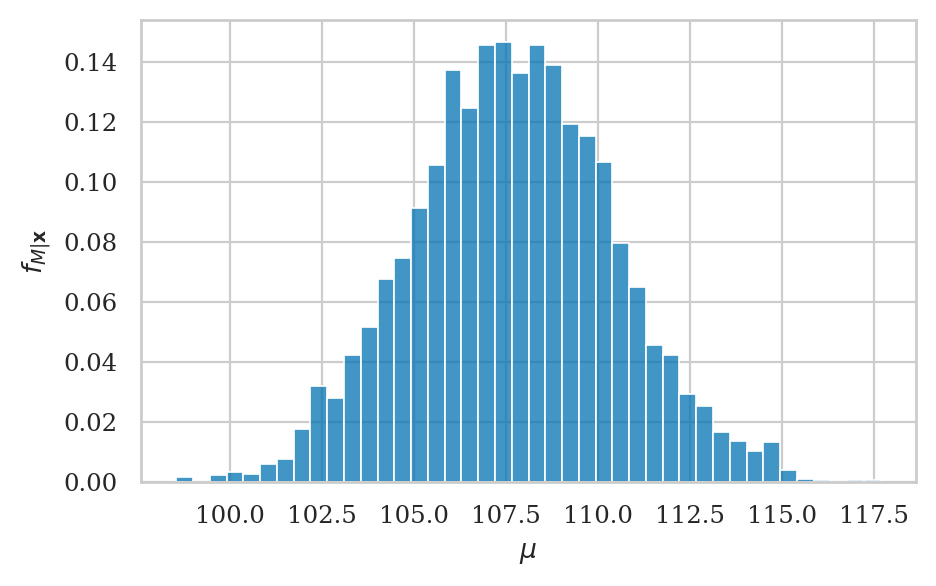
Visualize the posterior#

Histogram#

ax = sns.histplot(x=postM, stat="density")
ax.set_xlabel("$\\mu$")
ax.set_ylabel("$f_{M|\\mathbf{x}}$");

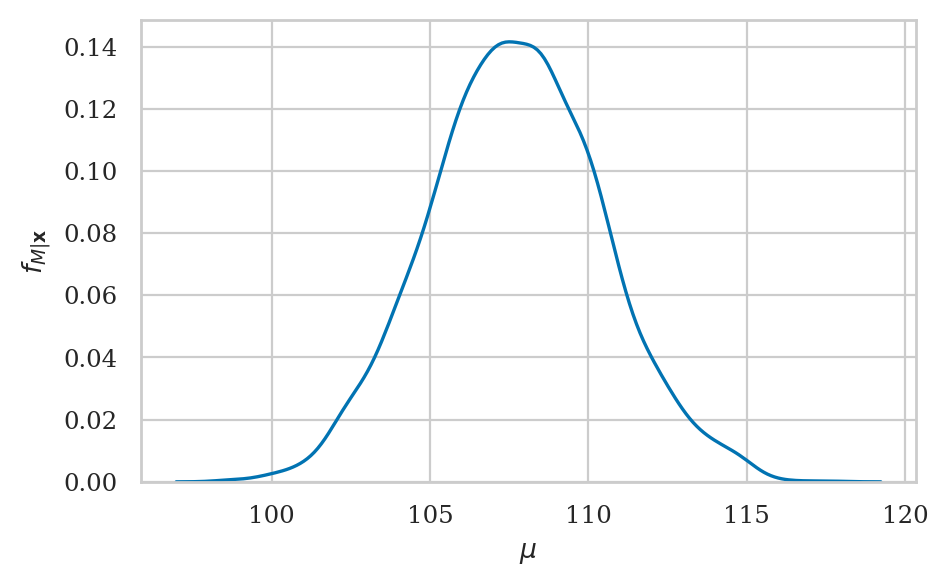
../_images/c7c3b2d7c84c3654732f070ee318ffb5109318e6d73a93c723623e11d40c5080.png

Kernel density plot#

ax = sns.kdeplot(x=postM)
ax.set_xlabel("$\\mu$")
ax.set_ylabel("$f_{M|\\mathbf{x}}$");

../_images/24933e59b111e3f8d50f23fe8613109fca41b095d70f25e5b96e6fe12bfe33bd.png

Summarize the posterior#

Posterior mean#

np.mean(postM)

107.71660366362643

Posterior standard deviation#

np.std(postM)

2.7321817530344927

Posterior median#

np.median(postM)

107.68693675071796

Posterior quartiles#

np.quantile(postM, [0.25, 0.5, 0.75])

array([105.89351247, 107.68693675, 109.56072492])

Posterior percentiles#

np.percentile(postM, [3, 97])

array([102.55117884, 112.96987424])

Posterior mode#

from ministats import mode_from_samples
mode_from_samples(postM)

107.51319922417586

Credible interval#

from ministats import hdi_from_samples
hdi_from_samples(postM, hdi_prob=0.9)

[103.09147595368688, 112.09548894571525]

Visualizing and interpreting posteriors#

import arviz as az

Example 1 continued: inferences about the biased coin#

Extracting samples (CUTTABLE)#

For the purpose of our data analysis, we don’t care about the chain and draw information and are only interested in in the variable P, which are the actual samples from the posterior. The easiest way to extract the samples from the posterior is to use the ArviZ helper method az.extract shown below.

postP = az.extract(idata1, var_names="P").values
postP.round(3)

array([0.761, 0.569, 0.776, ..., 0.602, 0.594, 0.663])

The call to the function az.extract selected the posterior group, then selected the variable P within the posterior group.

/CUTTABLE

Summarizing the posterior#

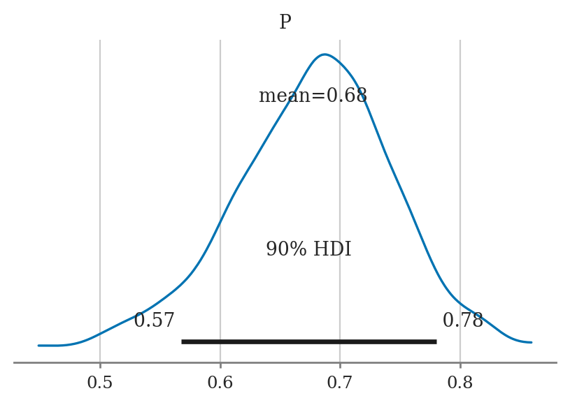
az.summary(idata1, kind="stats", hdi_prob=0.9)

	mean	sd	hdi_5%	hdi_95%
P	0.677	0.065	0.568	0.78

Plotting the posterior#

az.plot_posterior(idata1, var_names="P", hdi_prob=0.9);

../_images/893faf3efb068d6ba3143263c8bf9103cd42be703bd3b715c96ee0039d780d48.png

Options:

If multiple variables, you specify a list to var_names to select only certain variables to plot
Set the option point_estimate to "mode" or "median"
Add the option rope to draw region of practical equivalence, e.g., rope=[97,103]

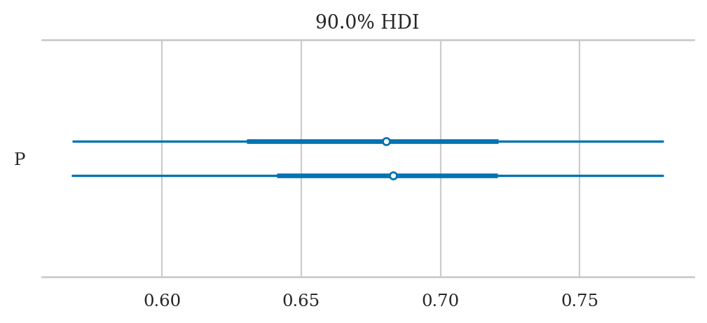
az.plot_forest(idata1, hdi_prob=0.9, figsize=(6,2.2));

../_images/5b5996b19e93feabc8360ccb2a861ac58c95e5244733cd8061473ac73cfbbcbb.png

Example 2 continued: inferences about the population mean#

Summarizing the posterior#

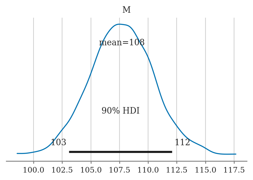
az.summary(idata2, kind="stats", hdi_prob=0.9)

	mean	sd	hdi_5%	hdi_95%
M	107.717	2.733	103.091	112.095

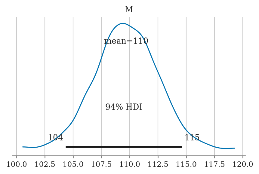
Plotting the posterior#

az.plot_posterior(idata2, var_names="M", hdi_prob=0.9);

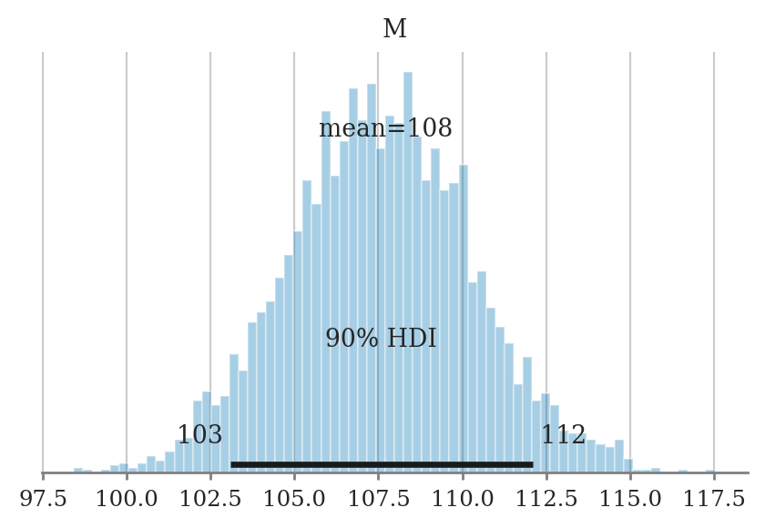
../_images/7a29ae1bab5fadd3a9e6b175118c365448d215cc74e18319a8529f1d9e56727d.png

az.plot_posterior(idata2, var_names="M", hdi_prob=0.9, kind="hist", bins=70);

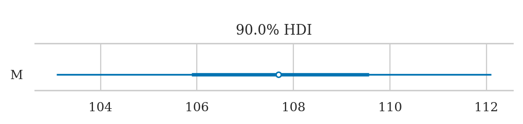
../_images/fbfdf41aa306e183ed5af737cd3d569177ad70d3dddb6b6189950625ee4bfd96.png

az.plot_forest(idata2, combined=True, hdi_prob=0.9, figsize=(6,0.6));

../_images/97d4be8183d12d290a6d7511eebb00d5a62246bf819b5ae7b47d1b7969dfac5b.png

Hypothesis testing#

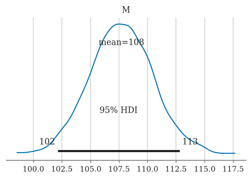
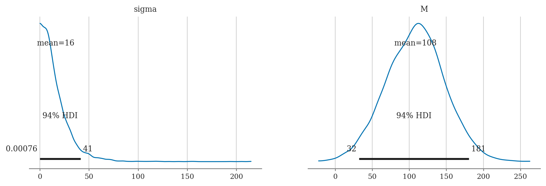
az.plot_posterior(idata2, hdi_prob=0.95);

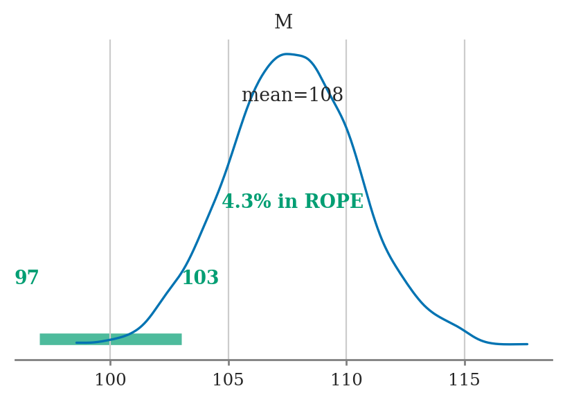
../_images/9d5b961b9d94549a84d221d12825bacbb04e275b0f7396fa5a9ea1cb44db3b3c.png

az.plot_posterior(idata2, hdi_prob="hide", rope=[97,103]);

../_images/162a274a0e903f03c9481dcdd99324237fcfa737dd20c2cd7df8077a1d922f34.png

Explanations#

Visualizing prior distributions#

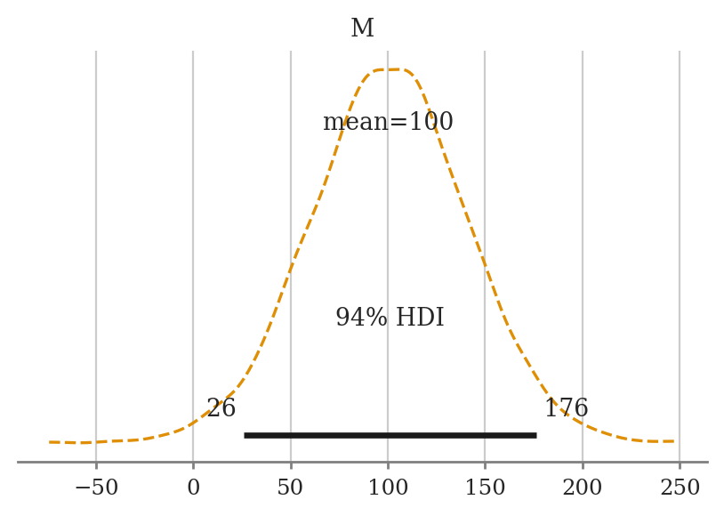
mod2.plot_priors(random_seed=43, color="C1", linestyle="dashed");

Sampling: [M]

../_images/acf9fcacce3e9fb1760d82e77da26c0ea07d1bd326c862a94b9153c845a3f67f.png

Bambi default priors#

iqs["iq"].mean(), iqs["iq"].std(ddof=0), 2.5*iqs["iq"].std(ddof=0)

(107.82333333333334, 15.812119472803834, 39.53029868200959)

mod2d = bmb.Model("iq ~ 1", family="gaussian", data=iqs)
mod2d

       Formula: iq ~ 1
        Family: gaussian
          Link: mu = identity
  Observations: 30
        Priors: 
    target = mu
        Common-level effects
            Intercept ~ Normal(mu: 107.8233, sigma: 39.5303)
        
        Auxiliary parameters
            sigma ~ HalfStudentT(nu: 4.0, sigma: 15.8121)

mod2d.build()
mod2d.plot_priors();

Sampling: [Intercept, sigma]

../_images/07723cc69e15cb9f9679a7d8826882770923754646be8546b663ccdb217b41e8.png

Groups are `Dataset` objects#

post1 = idata1["posterior"]
type(post1)

xarray.core.dataset.Dataset

# post1

post1.coords

Coordinates:
  * chain    (chain) int64 16B 0 1
  * draw     (draw) int64 8kB 0 1 2 3 4 5 6 7 ... 993 994 995 996 997 998 999

post1.data_vars

Data variables:
    P        (chain, draw) float64 16kB 0.7612 0.5686 0.7762 ... 0.5944 0.6632

Variables are `DataArray` objects#

Ps = post1["P"]  # == idata1["posterior"]["P"]
type(Ps)

xarray.core.dataarray.DataArray

# Ps

Ps.shape

(2, 1000)

Ps.name

'P'

Ps.to_dataframe()

		P
chain	draw
0	0	0.761228
	1	0.568612
	2	0.776170
	3	0.675721
	4	0.749423
...	...	...
1	995	0.639569
	996	0.665563
	997	0.601824
	998	0.594385
	999	0.663212

2000 rows × 1 columns

Ps.values

array([[0.76122756, 0.56861221, 0.77616961, ..., 0.70772348, 0.62878475,
        0.70789234],
       [0.68937002, 0.73226925, 0.67623114, ..., 0.60182373, 0.59438488,
        0.6632119 ]])

Ps.values.flatten()

array([0.76122756, 0.56861221, 0.77616961, ..., 0.60182373, 0.59438488,
       0.6632119 ])

MCMC diagnostics#

Trace plots#

There are several Arviz plots we can use to check if the Markov Chain Monte Carlo chains were sampling from the posterior as expected, or …

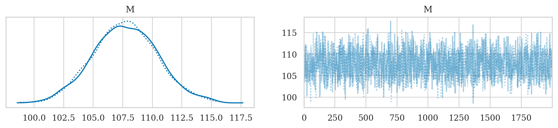
az.plot_trace(idata2);

../_images/8979dbfa273b87f35a440241e9ad18d80e0fc7a5dd2df3400a536038129c3376.png

Rank plots#

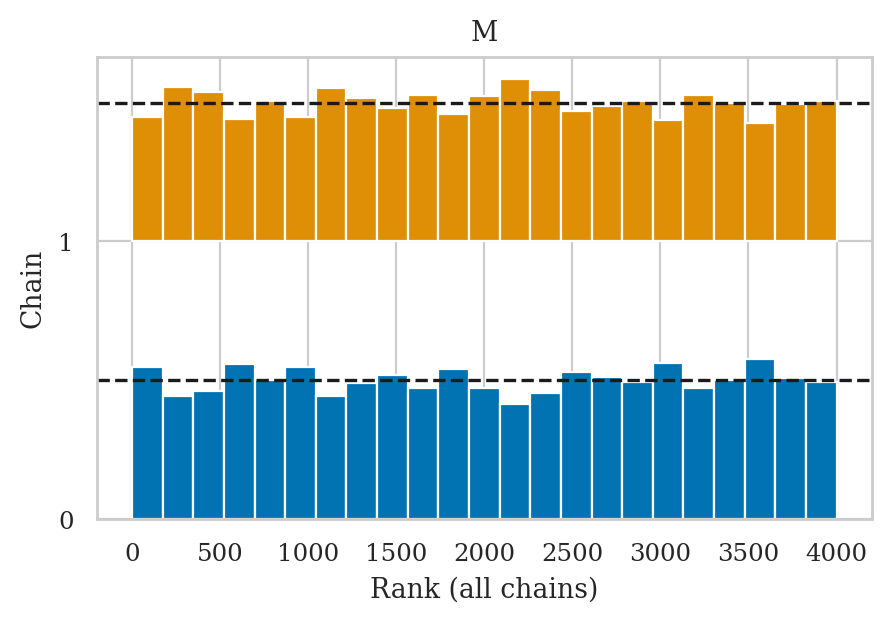
az.plot_rank(idata2);

../_images/6e336e46ec0dad0625c7b5b5efae3739c487bfd142645b3883746ffab272894a.png

? Autocorrelation plot ?#

https://python.arviz.org/en/stable/api/generated/arviz.plot_autocorr.html

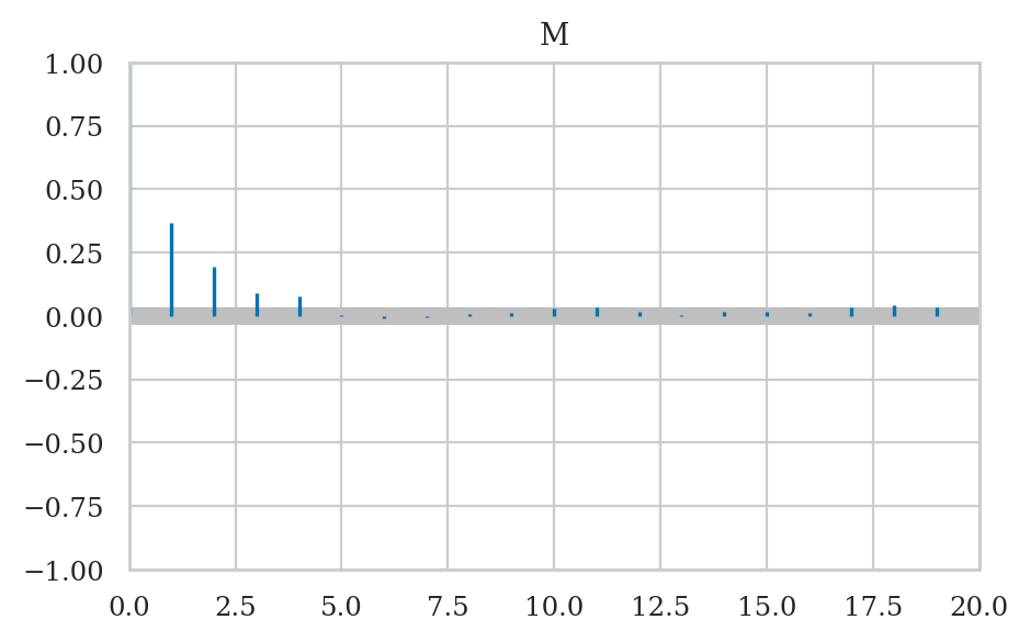
az.plot_autocorr(idata2, combined=True, max_lag=20);

../_images/49591e326f2bc9a9a0b74ecbbfd73f6ae623c75de5c3ce177b4f3c06a25dc360.png

Diagnostic summary#

az.summary(idata2, kind="stats")

	mean	sd	hdi_3%	hdi_97%
M	107.717	2.733	102.463	112.813

az.summary(idata2, kind="diagnostics")

	mcse_mean	mcse_sd	ess_bulk	ess_tail	r_hat
M	0.068	0.04	1625.0	2559.0	1.0

Bayesian workflow#

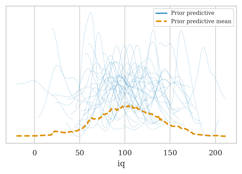
Prior predictive checks#

idata2_pri = mod2.prior_predictive(draws=50, random_seed=45)
az.plot_ppc(idata2_pri, group="prior");

Sampling: [M, iq]

../_images/3f7f942da86a9cfaf56c799daf36bff0657f997f6618518dc1352de499fa3cd1.png

idata2_pri['prior']["mu"].shape

(1, 50, 30)

idata2_pri['prior_predictive']["iq"].shape

(1, 50, 30)

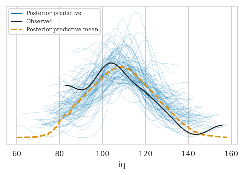
Posterior predictive checks#

# Randomly sample 200 from all available posterior mean
# draws_subset = np.random.choice(idata2["posterior"]["draw"].values, 50, replace=False)
draws_subset = np.random.choice(2000, 50, replace=False)
idata2_rep = idata2.sel(draw=draws_subset)
mod2.predict(idata2_rep, kind="response")
az.plot_ppc(idata2_rep, group="posterior")

<Axes: xlabel='iq'>

../_images/ea334a52ea53fa03bd03a5367b632b62d72fb15dba2d2da1e475945e4d47a12a.png

Fitting model to synthetic data#

np.random.seed(46)
from scipy.stats import norm
fakeiqs = norm(loc=110, scale=15).rvs(30)
fakeiqs = pd.DataFrame({"iq":fakeiqs})
fakeiqs["iq"].mean()

109.7132680142492

#######################################################
mod2f = bmb.Model(formula="iq ~ 1", family="gaussian",
                  priors=priors2, data=fakeiqs)
mod2f.set_alias({"Intercept": "M"})
idata2f = mod2f.fit(random_seed=42)

Initializing NUTS using jitter+adapt_diag...

Multiprocess sampling (2 chains in 2 jobs)

NUTS: [M]

Sampling 2 chains for 1_000 tune and 1_000 draw iterations (2_000 + 2_000 draws total) took 1 seconds.

We recommend running at least 4 chains for robust computation of convergence diagnostics

az.summary(idata2f, kind="stats")

	mean	sd	hdi_3%	hdi_97%
M	109.691	2.732	104.352	114.629

az.plot_posterior(idata2f);

../_images/b0b6625b358638569ef41383e8b7bb2b674491056ad94c4822001834a26196a6.png

Sensitivity analysis#

# TODO: reproduce sensitivity analysis from Secion 5.1

Iterative model building#

Discussion#

Other types of priors#

Conjugate priors#

Uninformative priors#

Software for Bayesian inference#

Computational cost#

Reporting Bayesian results#

Model predictions (BONUS TOPIC)#

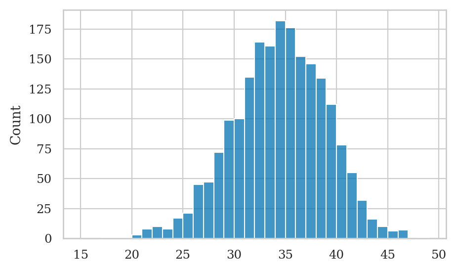
Coin toss predictions#

Let’s generate some observations form the posterior predictive distribution.

idata1_pred = idata1.copy()
# MAYBE: alt notation _rep instead of _pred ?
mod1.predict(idata1_pred, kind="response")
ctosses_pred = az.extract(idata1_pred,
                          group="posterior_predictive",
                          var_names=["ctoss"]).values
numheads_pred = ctosses_pred.sum(axis=0)

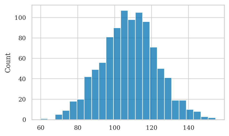
sns.histplot(x=numheads_pred, bins=range(15,50));

../_images/81122fdfb715c49620c85d1624066213026d35be7696d42f23c3e5aacdd54f21.png

IQ predictions#

## Can't use Bambi predict because of issue
## https://github.com/bambinos/bambi/issues/850
# idata2_pred = mod2.predict(idata2, kind="response", inplace=False)
# preds2 = az.extract(idata2_pred, group="posterior", var_names=["mu"]).values.flatten()

from scipy.stats import norm

sigma = 15  # known population standard deviation

iq_preds = []
np.random.seed(42)
for i in range(1000):
    mu_post = np.random.choice(postM)
    iq_pred = norm(loc=mu_post, scale=sigma).rvs(1)[0]
    iq_preds.append(iq_pred)

sns.histplot(x=iq_preds);

../_images/711a0613b40272424a100645efc277219263b29a808ea1cecde3a9308530884a.png

Exercises#

TODO: repeat exercises form Sec 5.1 using Bambi and ArviZ

Exercise A#

Reproduce the analysis of the IQ scores data from Example 2, but this time use a model with Bambi default priors.

a) Plot the priors using plot_priors.
b) Compute the posterior mean, std, and a 90% hdi.
c) Compare your result in (b) to the results we obtained from Example 2.

mod2d = bmb.Model("iq ~ 1", family="gaussian", data=iqs)
mod2d.set_alias({"Intercept": "M"})
mod2d.build()
mod2d.plot_priors();

Sampling: [M, sigma]

../_images/19136f51434333241911fa36e4185d4a5351b42c9e5b7ea069472b22f2ff10ff.png

idata2d = mod2d.fit(draws=2000, random_seed=42)
az.summary(idata2d, var_names="M", kind="stats", hdi_prob=0.9)

Initializing NUTS using jitter+adapt_diag...

/opt/hostedtoolcache/Python/3.10.17/x64/lib/python3.10/site-packages/pytensor/link/c/cmodule.py:2959: UserWarning: PyTensor could not link to a BLAS installation. Operations that might benefit from BLAS will be severely degraded.
This usually happens when PyTensor is installed via pip. We recommend it be installed via conda/mamba/pixi instead.
Alternatively, you can use an experimental backend such as Numba or JAX that perform their own BLAS optimizations, by setting `pytensor.config.mode == 'NUMBA'` or passing `mode='NUMBA'` when compiling a PyTensor function.
For more options and details see https://pytensor.readthedocs.io/en/latest/troubleshooting.html#how-do-i-configure-test-my-blas-library
  warnings.warn(
Multiprocess sampling (2 chains in 2 jobs)

NUTS: [sigma, M]

Sampling 2 chains for 1_000 tune and 2_000 draw iterations (2_000 + 4_000 draws total) took 2 seconds.

We recommend running at least 4 chains for robust computation of convergence diagnostics

	mean	sd	hdi_5%	hdi_95%
M	107.768	3.021	102.903	112.743

az.summary(idata2, kind="stats", hdi_prob=0.9)

	mean	sd	hdi_5%	hdi_95%
M	107.717	2.733	103.091	112.095

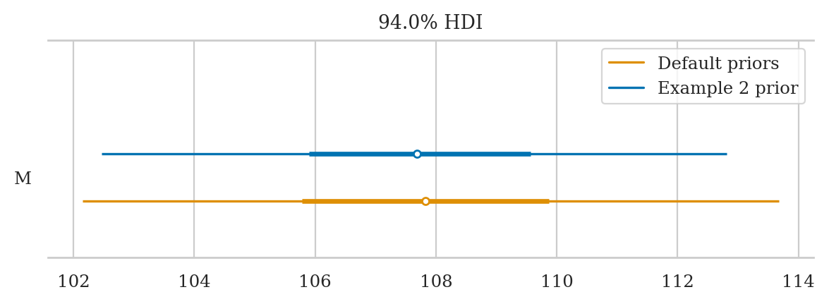
az.plot_forest(data=[idata2, idata2d],
               model_names=["Example 2 prior", "Default priors"],
               var_names="M", combined=True, figsize=(7,2));

../_images/7a0ccfb1de0dd98466ee3f2979e7c97ae303471862ab77f4445e9f52a119cd16.png

Exercise B#

Repeat the analysis in Example 2, but this time use the exponential prior \(\text{Expon}(\lambda=0.1)\) on the parameter sigma. Calculate:

a) Plot the priors using plot_priors.
b) Compute posterior mean of M and sigma.
c) Compute the posterior median of M and sigma.
d) Compute 90% credible interval for M and sigma.

import bambi as bmb
priors2e = {
    "Intercept": bmb.Prior("Normal", mu=100, sigma=40),
    "sigma": bmb.Prior("Exponential", lam=0.1),
}

mod2e = bmb.Model(formula="iq ~ 1",
                  family="gaussian",
                  link="identity",
                  priors=priors2e,
                  data=iqs)
mod2e.set_alias({"Intercept": "M"})

mod2e.build()
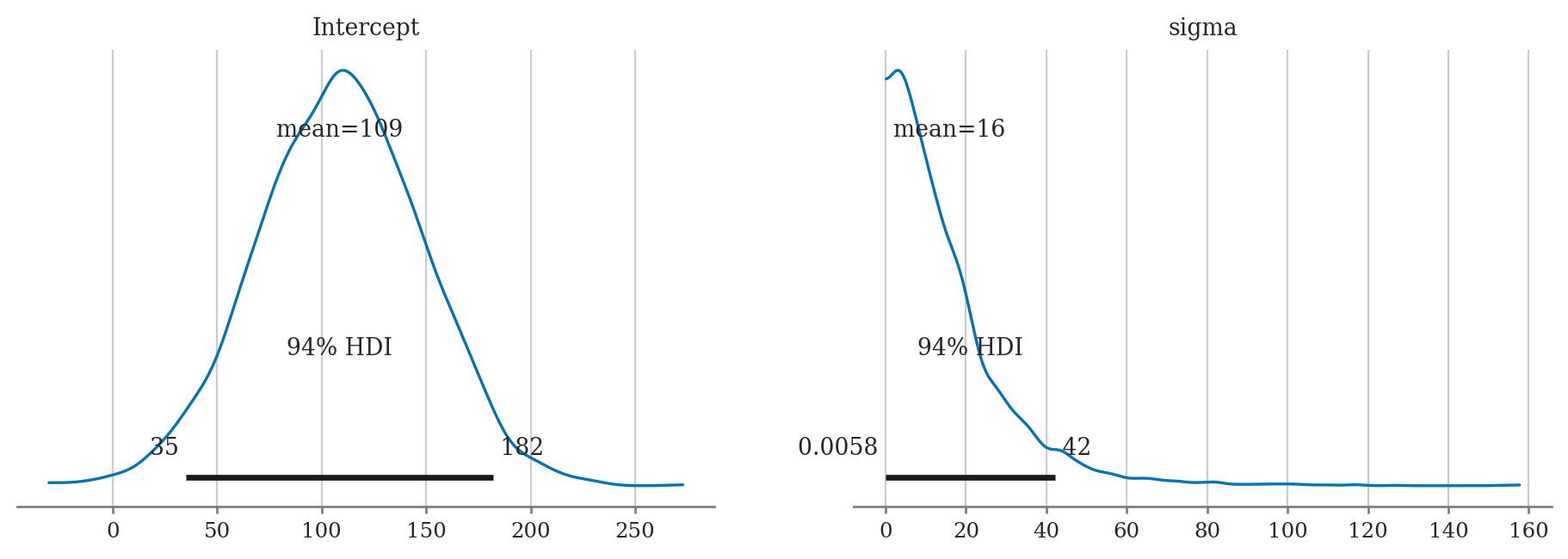
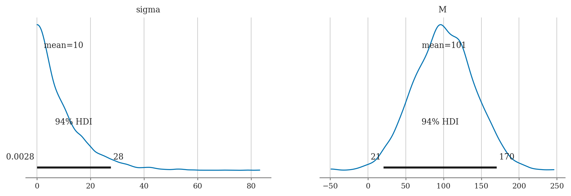
mod2e.plot_priors();

Sampling: [M, sigma]

../_images/bf14d93f00a5f4d34cae127fe8c096f3a303c591faf0bfd238a938dc4dd647a2.png

# idata2e = mod2e.fit(random_seed=42)
# az.plot_posterior(idata2e)

# JOINT PLOT
# M_samples = idata2e.posterior['M'].values.flatten()
# sigma_samples = idata2e.posterior['sigma'].values.flatten()
# sns.kdeplot(x=M_samples, y=sigma_samples, fill=True)
# plt.xlabel('M')
# plt.ylabel('Sigma')
# plt.title('Density Plot of Mean vs Sigma')

Exercise C#

Links#

TODO

Section 5.2 — Bayesian inference computations

Contents

Section 5.2 — Bayesian inference computations#

Notebook setup#

Definitions#

Posterior inference using MCMC estimation#

Bayesian inference using Bambi#

Example 1: estimating the probability of a bias of a coin#

Data#

Model#

Fitting the model#

Exploring InferenceData objects#

Extracting the samples from the posterior#

Visualize the posterior#

Histogram#

Kernel density plot#

Summarize the posterior#

Posterior mean#

Posterior standard deviation#

Posterior median#

Posterior quartiles#

Posterior percentiles#

Posterior mode#

Credible interval#

Example 2: estimating the IQ score#

Data#

Model#

Fitting the model#

Extract the samples from the posterior#

Visualize the posterior#

Histogram#

Kernel density plot#

Summarize the posterior#

Posterior mean#

Posterior standard deviation#

Posterior median#

Posterior quartiles#

Posterior percentiles#

Posterior mode#

Credible interval#

Visualizing and interpreting posteriors#

Example 1 continued: inferences about the biased coin#

Extracting samples (CUTTABLE)#

Summarizing the posterior#

Plotting the posterior#

Example 2 continued: inferences about the population mean#

Summarizing the posterior#

Plotting the posterior#

Hypothesis testing#

Explanations#

Visualizing prior distributions#

Bambi default priors#

More about inference data objects#

Groups are Dataset objects#

Variables are DataArray objects#

MCMC diagnostics#

Trace plots#

Rank plots#

? Autocorrelation plot ?#

Diagnostic summary#

Bayesian workflow#

Prior predictive checks#

Posterior predictive checks#

Fitting model to synthetic data#

Sensitivity analysis#

Iterative model building#

Discussion#

Other types of priors#

Conjugate priors#

Uninformative priors#

Software for Bayesian inference#

Computational cost#

Reporting Bayesian results#

Model predictions (BONUS TOPIC)#

Coin toss predictions#

IQ predictions#

Exercises#

Exercise A#

Exercise B#

Exercise C#

Exploring `InferenceData` objects#

Groups are `Dataset` objects#

Variables are `DataArray` objects#