Section 2.3 — Inventory of discrete distributions#
This notebook contains all the code examples from Section 2.3 Inventory of discrete distributions of the No Bullshit Guide to Statistics.
Notebook setup#
# Ensure required Python modules are installed
%pip install --quiet numpy scipy seaborn ministats
[notice] A new release of pip is available: 26.1.1 -> 26.1.2
[notice] To update, run: pip install --upgrade pip
Note: you may need to restart the kernel to use updated packages.
# Load Python modules
import numpy as np
import seaborn as sns
import matplotlib.pyplot as plt
from ministats import plot_pmf
# Figures setup
plt.clf()  # needed otherwise `sns.set_theme` doesn't work
sns.set_theme(
    context="paper",
    style="whitegrid",
    palette="colorblind",
    rc={"font.family": "serif",
        "font.serif": ["Palatino", "DejaVu Serif", "serif"],
        "figure.figsize": (6,2)},
)
%config InlineBackend.figure_format = "retina"
<Figure size 640x480 with 0 Axes>
# Simple float __repr__
import numpy as np
if int(np.__version__.split(".")[0]) >= 2:
    np.set_printoptions(legacy='1.25')

# set random seed for repeatability
np.random.seed(42)
Discrete uniform distribution#
from scipy.stats import randint

alpha = 1
beta = 4
rvR = randint(alpha, beta+1)
Note the +1 we added to the second argument.
rvR.mean()
2.5
rvR.var()
1.25
The limits of the sample space of the random variable rvR
can be obtained by calling its .support() method.
Probability mass function#
plot_pmf(rvR, xlims=[0,8+1]);
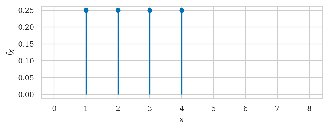
rvR.support()
(1, 4)
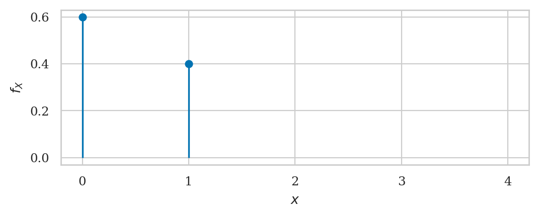
Bernoulli distribution#
from scipy.stats import bernoulli

rvB = bernoulli(p=0.4)
rvB.support()
(0, 1)
rvB.mean(), rvB.var()
(0.4, 0.24)
rvB.rvs(10)
array([0, 1, 1, 0, 0, 0, 0, 1, 1, 1])
plot_pmf(rvB, xlims=[0,5]);
Mathematical interlude: counting combinations#
Factorials#
TODO explain + math formula
from scipy.special import factorial

factorial(4)
24.0
# # ALT.
# from math import factorial
# factorial(4)
The factorial of \(0\) is defined as 1: \(0!=1\).
factorial(0)
1.0
The factorial function grows grows very quickly:
[factorial(n) for n in [5, 6, 7, 8, 9, 10, 11, 12, 13]]
[120.0,
 720.0,
 5040.0,
 40320.0,
 362880.0,
 3628800.0,
 39916800.0,
 479001600.0,
 6227020800.0]
Combinations#
TODO explain + math formula
from scipy.special import comb

comb(5, 2)
10.0
from itertools import combinations

list(combinations({1,2,3,4,5}, 2))
[(1, 2),
 (1, 3),
 (1, 4),
 (1, 5),
 (2, 3),
 (2, 4),
 (2, 5),
 (3, 4),
 (3, 5),
 (4, 5)]
Exercises#
from scipy.special import comb

comb(12,6)
924.0
from scipy.special import comb

comb(52,5)
2598960.0
Links#
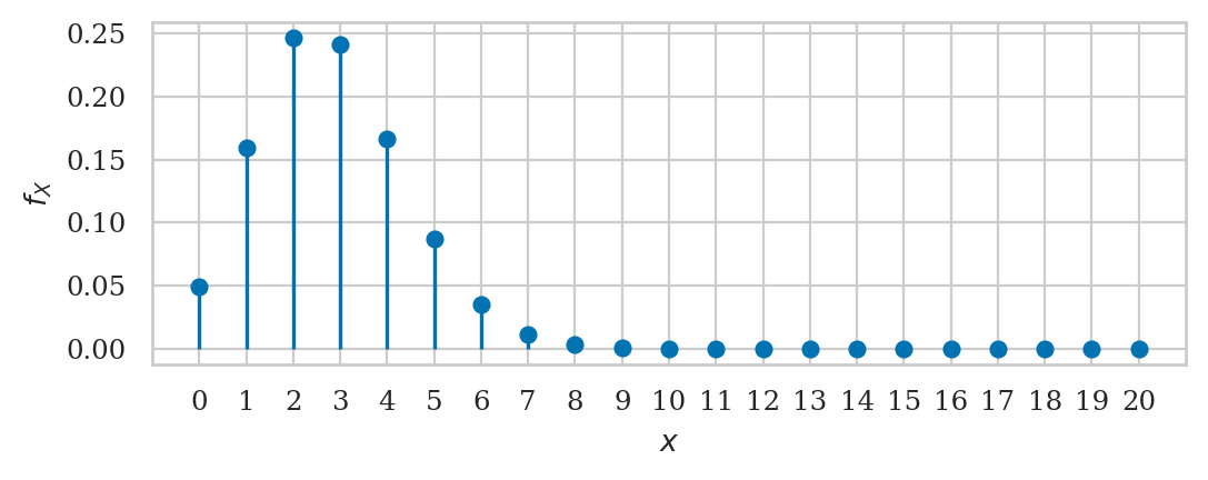
Binomial distribution#
We’ll use the name rvX because rvB was already used for the Bernoulli random variable above.
from scipy.stats import binom

n = 20
p = 0.14
rvX = binom(n,p)
rvX.support()
(0, 20)
rvX.mean(), rvX.var()
(2.8000000000000003, 2.4080000000000004)
plot_pmf(rvX, xlims=[0,21]);
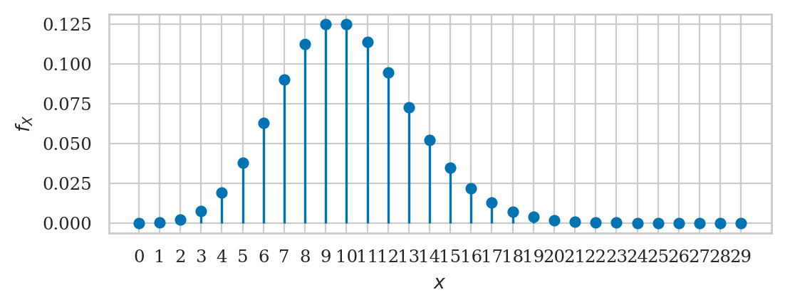
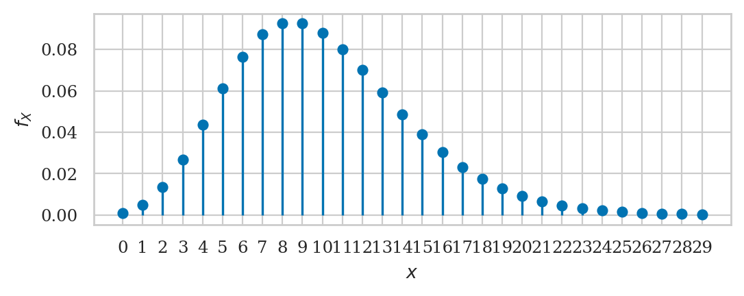
Poisson distribution#
from scipy.stats import poisson
lam = 10
rvP = poisson(lam)
rvP.pmf(8)
0.11259903214902009
rvP.cdf(8)
0.3328196787507191
## ALT. way to compute the value F_P(8) =
# sum([rvP.pmf(x) for x in range(0,8+1)])
plot_pmf(rvP, xlims=[0,30]);
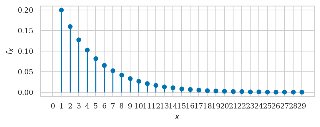
Geometric distribution#
from scipy.stats import geom

rvG = geom(p = 0.2)
rvG.support()
(1, inf)
rvG.mean(), rvG.var()
(5.0, 20.0)
plot_pmf(rvG, xlims=[0,30]);
Negative binomial distribution#
from scipy.stats import nbinom

r = 10
p = 0.5
rvN = nbinom(r,p)
rvN.support()
(0, inf)
rvN.mean(), rvN.var()
(10.0, 20.0)
plot_pmf(rvN, xlims=[0,30]);
Computer models for discrete distributions#
TODO table models
TODO table methods
Building computer models for random variables#
# import the model family
from scipy.stats import randint

# choose parameters
alpha = 1  # start at 1
beta = 4   # stop at 4

# create the rv object
rvR = randint(alpha, beta+1)
Note the +1 we added to the second argument.
rvR.mean()
2.5
# verify using formula
(alpha + beta) / 2
2.5
rvR.var()
1.25
# verify using formula
((beta + 1 - alpha)**2 - 1) / 12
1.25
rvR.std()
1.118033988749895
The limits of the sample space of the random variable rvR
can be obtained by calling its .support() method.
rvR.support()
(1, 4)
Probability calculations#
rvR.pmf(1) + rvR.pmf(2) + rvR.pmf(3)
0.75
[rvR.pmf(r) for r in range(1,3+1)]
[0.25, 0.25, 0.25]
sum([rvR.pmf(r) for r in range(1,3+1)])
0.75
rvR.cdf(3)
0.75
Plotting distributions#
Probability mass function#
To create a stem-plot of the probability mass function \(f_R\), we can use the following three-step procedure:
Create a range of inputs
rsfor the plot.Compute the value of \(f_R =\)
rvRfor each of the inputs and store the results as list of valuesfRs.Plot the values
fRsby calling the functionplt.stem(rs, fRs).
import matplotlib.pyplot as plt

rs = range(0, 8+1)
fRs = rvR.pmf(rs)
fRs = np.where(fRs == 0, np.nan, fRs)  # set zero fRs to np.nan
plt.stem(rs, fRs, basefmt=" ");
plt.xlabel("$r$")
plt.ylabel("$f_R$")
Text(0, 0.5, '$f_R$')

Note, we used the np.where statement
to replace zero entries in the list fRs
to the special Not a Number (np.nan) values,
which excludes them from the plot.
This is arguably a cleaner representation of the PMF plot:
the function is only defined for the sample space \(\mathcal{R} = \{1,2,3,4\}\).
An alternative ,,,
# ALT. using helper function
from ministats import plot_pmf

plot_pmf(rvR, xlims=[0,8+1], rv_name="R");
# Uncomment and run this to see the `plot_pmf` source code
# %psource plot_pmf
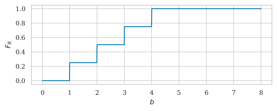
Cumulative distribution function#
import numpy as np
import seaborn as sns

bs = np.linspace(0, 8, 1000)
FRs = rvR.cdf(bs)
sns.lineplot(x=bs, y=FRs);
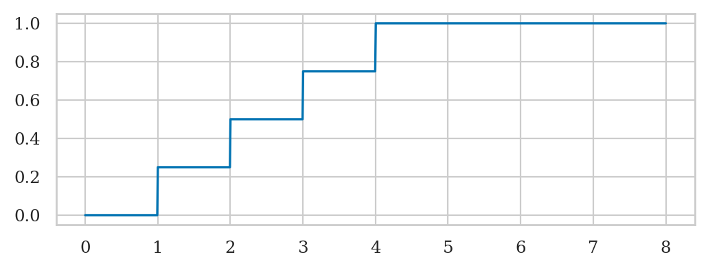
# ALT. using helper function
from ministats import plot_cdf

plot_cdf(rvR, xlims=[0,8], rv_name="R");
Generating random observations#
Let’s generate 10 random observations from random variable rvR:
np.random.seed(43)

rvR.rvs(10)
array([1, 1, 4, 2, 2, 3, 1, 4, 2, 4])
Explanations#
Binomial coefficient formula explained#
n = 6
[int(comb(n,k)) for k in range(0,n+1)]
[1, 6, 15, 20, 15, 6, 1]
We can draw Pascal’s triangle
by by repeating the above calculation for several values of n.
for n in range(0,10):
    row_ints = [int(comb(n,k)) for k in range(0,n+1)]
    row_str = str(row_ints)
    row_str = row_str.replace("[","").replace("]","").replace(",", "  ")
    row_str = row_str.center(60)
    print(row_str)
                             1
                           1   1
                         1   2   1
                       1   3   3   1
                     1   4   6   4   1
                  1   5   10   10   5   1
                1   6   15   20   15   6   1
             1   7   21   35   35   21   7   1
           1   8   28   56   70   56   28   8   1
       1   9   36   84   126   126   84   36   9   1
Geometric sums#
r = 0.3
sum([r**n for n in range(0,100)])
1.4285714285714286
1 / (1 - r)
1.4285714285714286
Discussion#
Relations between distributions#
Exercises#
Exercise XX#
from scipy.stats import poisson
lam = 20
rvH = poisson(lam)
# a) Pr(H in {20,21,22})
rvH.pmf(20) + rvH.pmf(21) + rvH.pmf(22)
0.2503540762867847
# b) Pr({16≤H≤24})
rvH.cdf(24) - rvH.cdf(16-1)
0.6867142435340193
# c) F_H^{-1}(0.95)
rvH.ppf(0.95)
28.0