Section 4.2 — Multiple linear regression#
This notebook contains the code examples from Section 4.2 Multiple linear regression from the No Bullshit Guide to Statistics.
Notebook setup#
# Ensure required Python modules are installed
%pip install --quiet numpy scipy seaborn statsmodels ministats
[notice] A new release of pip is available: 26.1.1 -> 26.1.2
[notice] To update, run: pip install --upgrade pip
Note: you may need to restart the kernel to use updated packages.
# load Python modules
import numpy as np
import pandas as pd
import seaborn as sns
import matplotlib.pyplot as plt
# Figures setup
plt.clf()  # needed otherwise `sns.set_theme` doesn't work
sns.set_theme(
    context="paper",
    style="whitegrid",
    palette="colorblind",
    rc={"font.family": "serif",
        "font.serif": ["Palatino", "DejaVu Serif", "serif"],
        "figure.figsize": (5,2.3)},
)
%config InlineBackend.figure_format = "retina"
<Figure size 640x480 with 0 Axes>
# Simple float __repr__
if int(np.__version__.split(".")[0]) >= 2:
    np.set_printoptions(legacy='1.25')

# set random seed for repeatability
np.random.seed(42)
# Download datasets/ directory if necessary
from ministats import ensure_datasets
ensure_datasets()
datasets/ directory already exists.
Definitions#
TODO
Doctors dataset#
doctors = pd.read_csv("datasets/doctors.csv")
doctors.shape
(156, 9)
doctors.head()
| permit | loc | work | hours | caf | alc | weed | exrc | score | |
|---|---|---|---|---|---|---|---|---|---|
| 0 | 93273 | rur | hos | 21 | 2 | 0 | 5.0 | 0.0 | 63 |
| 1 | 90852 | urb | cli | 74 | 26 | 20 | 0.0 | 4.5 | 16 |
| 2 | 92744 | urb | hos | 63 | 25 | 1 | 0.0 | 7.0 | 58 |
| 3 | 73553 | urb | eld | 77 | 36 | 4 | 0.0 | 2.0 | 55 |
| 4 | 82441 | rur | cli | 36 | 22 | 9 | 0.0 | 7.5 | 47 |
Multiple linear regression model#
\(\newcommand{\Err}{ {\Large \varepsilon}}\)
where \(p\) is the number of predictors and \(\Err\) represents Gaussian noise \(\Err \sim \mathcal{N}(0,\sigma)\).
Model assumptions#
(LIN)
(INDEPɛ)
(NORMɛ)
(EQVARɛ)
(NOCOL)
Example: linear model for doctors’ sleep scores#
We want to know the influence of drinking alcohol, smoking weed, and exercise on sleep score?
import statsmodels.formula.api as smf
formula = "score ~ 1 + alc + weed + exrc"
lm2 = smf.ols(formula, data=doctors).fit()
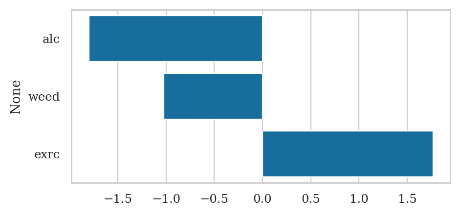
lm2.params
Intercept    60.452901
alc          -1.800101
weed         -1.021552
exrc          1.768289
dtype: float64
sns.barplot(x=lm2.params.values[1:],
            y=lm2.params.index[1:]);
Partial regression plots#
Partial regression plot for the predictor alc#
Step 1: Obtain the data for the x-axis,
residuals of the model alc ~ 1 + others
#######################################################
lm_alc = smf.ols("alc~1+weed+exrc", data=doctors).fit()
xrs = lm_alc.resid
Step 2: Obtain the data for the y-axis,
residuals of the model score ~ 1 + others
#######################################################
lm_score=smf.ols("score~1+weed+exrc",data=doctors).fit()
yrs = lm_score.resid
Step 3: Fit a linear model for the y-residuals versus the x-residuals.
dfrs = pd.DataFrame({"xrs": xrs, "yrs": yrs})
lm_resids = smf.ols("yrs ~ 1 + xrs", data=dfrs).fit()
Step 4: Draw a scatter plot of the residuals and the best-fitting linear model to the residuals.
from ministats import plot_reg

ax = sns.scatterplot(x=xrs, y=yrs, color="C0")
plot_reg(lm_resids, ax=ax);
ax.set_xlabel("alc~1+weed+exrc  residuals")
ax.set_ylabel("score~1+weed+exrc  residuals")
ax.set_title("Partial regression plot for `alc`");
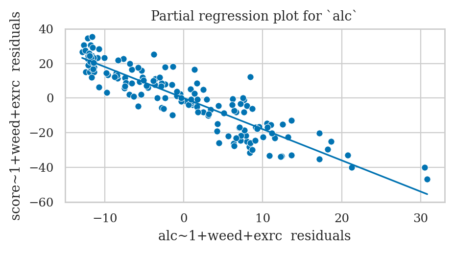
The slope parameter for the residuals model
is the same as the slope parameter of the alc predictor in the original model lm2.
lm_resids.params["xrs"], lm2.params["alc"]
(-1.8001013152459409, -1.8001013152459384)
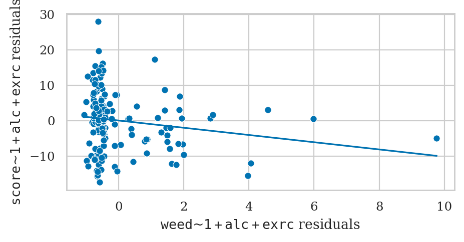
Partial regression plot for the predictor weed#
from ministats import plot_partreg
plot_partreg(lm2, pred="weed");
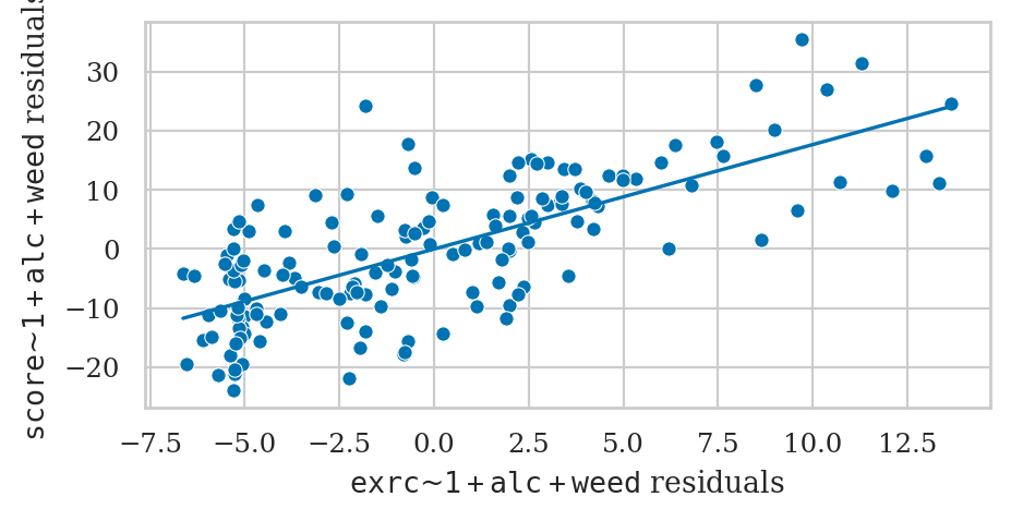
Partial regression plot for the predictor exrc#
plot_partreg(lm2, pred="exrc");
(BONUS TOPIC) Partial regression plots using statsmodels#
The function plot_partregress defined in statsmodels.graphics.api
performs the same steps as the function plot_partreg we used above.
but is a little more awkward to use.
When calling the function plot_partregress,
you must provide the following arguments:
the outcome variable (
endog)the predictor you’re interested in (
exog_i)the predictors you want to regress out (
exog_others)the data frame that contains all these variable (
data)
from statsmodels.graphics.api import plot_partregress

with plt.rc_context({"figure.figsize":(12,3)}):
    fig, (ax1, ax2, ax3) = plt.subplots(1,3, sharey=True)
    plot_partregress("score", "alc",  exog_others=["weed", "exrc"], data=doctors, obs_labels=False, ax=ax1)
    plot_partregress("score", "weed", exog_others=["alc",  "exrc"], data=doctors, obs_labels=False, ax=ax2)
    plot_partregress("score", "exrc", exog_others=["alc",  "weed"], data=doctors, obs_labels=False, ax=ax3)
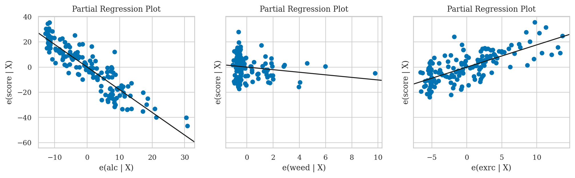
The notation \(|\textrm{X}\) you see in the axis labels stands for “given all other predictors,”
and is different for each subplot.
For example,
in the leftmost partial regression plot,
the predictor we are focussing on is alc,
so the other variables (\(|\textrm{X}\)) are weed and exrc.
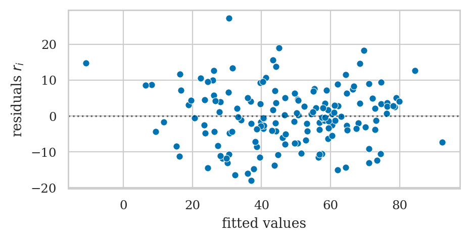
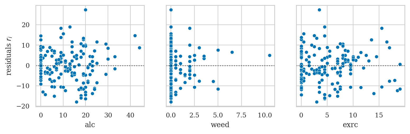
Plot residuals#
from ministats import plot_resid
plot_resid(lm2);
fig, (ax1,ax2,ax3) = plt.subplots(1, 3, sharey=True, figsize=(9,2.5))
plot_resid(lm2, pred="alc",  ax=ax1)
plot_resid(lm2, pred="weed", ax=ax2)
plot_resid(lm2, pred="exrc", ax=ax3);
Model summary table#
lm2.summary()
| Dep. Variable: | score | R-squared: | 0.842 |
|---|---|---|---|
| Model: | OLS | Adj. R-squared: | 0.839 |
| Method: | Least Squares | F-statistic: | 270.3 |
| Date: | Sun, 31 May 2026 | Prob (F-statistic): | 1.05e-60 |
| Time: | 22:36:35 | Log-Likelihood: | -547.63 |
| No. Observations: | 156 | AIC: | 1103. |
| Df Residuals: | 152 | BIC: | 1115. |
| Df Model: | 3 | ||
| Covariance Type: | nonrobust |
| coef | std err | t | P>|t| | [0.025 | 0.975] | |
|---|---|---|---|---|---|---|
| Intercept | 60.4529 | 1.289 | 46.885 | 0.000 | 57.905 | 63.000 |
| alc | -1.8001 | 0.070 | -25.726 | 0.000 | -1.938 | -1.662 |
| weed | -1.0216 | 0.476 | -2.145 | 0.034 | -1.962 | -0.081 |
| exrc | 1.7683 | 0.138 | 12.809 | 0.000 | 1.496 | 2.041 |
| Omnibus: | 1.140 | Durbin-Watson: | 1.828 |
|---|---|---|---|
| Prob(Omnibus): | 0.565 | Jarque-Bera (JB): | 0.900 |
| Skew: | 0.182 | Prob(JB): | 0.638 |
| Kurtosis: | 3.075 | Cond. No. | 31.2 |
Notes:
[1] Standard Errors assume that the covariance matrix of the errors is correctly specified.
Explanations#
Nonlinear terms in linear regression#
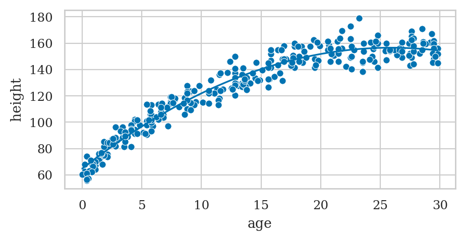
Example: polynomial regression#
howell30 = pd.read_csv("datasets/howell30.csv")
len(howell30)
298
# Fit quadratic model
formula2 = "height ~ 1 + age + np.square(age)"
lmq = smf.ols(formula2, data=howell30).fit()
lmq.params
Intercept         64.784755
age                7.086471
np.square(age)    -0.136775
dtype: float64
# Plot the data
sns.scatterplot(data=howell30, x="age", y="height");

# Plot the best-fit quadratic model
intercept, b_lin, b_quad = lmq.params
ages = np.linspace(0.1, howell30["age"].max())
heighthats = intercept + b_lin*ages + b_quad*ages**2
sns.lineplot(x=ages, y=heighthats, color="b");

# ALT. using `plot_reg` function
from ministats import plot_reg
plot_reg(lmq);
Feature engineering and transformed variables#
Bonus example: polynomial regression up to degree 3#
formula3 = "height ~ 1 + age + np.power(age,2) + np.power(age,3)"
exlm3 = smf.ols(formula3, data=howell30).fit()
exlm3.params
Intercept           63.367775
age                  7.699216
np.power(age, 2)    -0.188982
np.power(age, 3)     0.001165
dtype: float64
sns.scatterplot(data=howell30, x="age", y="height")
sns.lineplot(x=ages, y=exlm3.predict({"age":ages}));

Discussion#
Exercises#
Exercise E??: marketing dataset#
marketing = pd.read_csv("datasets/exercises/marketing.csv")
formula_mkt = "sales ~ 1 + youtube + facebook + newspaper"
lm_mkt2 = smf.ols(formula_mkt, data=marketing).fit()
lm_mkt2.params
Intercept    3.526667
youtube      0.045765
facebook     0.188530
newspaper   -0.001037
dtype: float64