Section 2.5 — Multiple continuous random variables#
This notebook contains all the code examples from Section 2.5 Multiple continuous random variables of the No Bullshit Guide to Statistics.
Notebook setup#
We’ll start by importing the Python modules we’ll need for this notebook.
# Ensure required Python modules are installed
%pip install --quiet numpy scipy seaborn ministats
[notice] A new release of pip is available: 26.1.1 -> 26.1.2
[notice] To update, run: pip install --upgrade pip
Note: you may need to restart the kernel to use updated packages.
# load Python modules
import numpy as np
import seaborn as sns
import matplotlib.pyplot as plt
# Figures setup
plt.clf()  # needed otherwise `sns.set_theme` doesn't work
sns.set_theme(
    context="paper",
    style="whitegrid",
    palette="colorblind",
    rc={"font.family": "serif",
        "font.serif": ["Palatino", "DejaVu Serif", "serif"],
        "figure.figsize": (7,2)},
)
%config InlineBackend.figure_format = "retina"
<Figure size 640x480 with 0 Axes>
# Simple float __repr__
import numpy as np
if int(np.__version__.split(".")[0]) >= 2:
    np.set_printoptions(legacy='1.25')
Definitions#
Random variables#
random variable \(X\): a quantity that can take on different values.
sample space \(\mathcal{X}\): describes the set of all possible outcomes of the random variable \(X\).
outcome: a particular value \(\{X = x\}\) that can occur as a result of observing the random variable \(X\).
event subset of the sample space \(\{a \leq X \leq b\}\) that can occur as a result of observing the random variable \(X\).
\(f_X\): the probability density function (PDF) is a function that assigns probabilities to the different outcome in the sample space of a random variable. The probability distribution function of the random variable \(X\) is a function of the form \(f_X: \mathcal{X} \to \mathbb{R}\).
Multiple random variables#
Example 3: bivariate normal distribution#
TODO: formula for general bivarate normal
from scipy.stats import multivariate_normal

# Model parameters
muX, muY, sigmaX, sigmaY, rho = 10, 5, 3, 1, 0.75

# The mean vector
mu = [muX, muY]

# The covariance matrix
Sigma = [[         sigmaX**2,   rho*sigmaX*sigmaY ],
         [ rho*sigmaX*sigmaY,           sigmaY**2 ]]


# Computer model for the bivariate normal random variable
rvXY = multivariate_normal(mu, Sigma)
rvXY.pdf((10,5))
0.08020655225672235
Probability of the event \(\{10 \leq X \leq 14, 5 \leq Y \leq 7\}\).
from scipy.integrate import dblquad

def fYX(y,x):
    """
    Adapter function because `dblquad` expects the function
    we're integrating to be of the form f(y,x), and not f(x,y).
    """
    return rvXY.pdf([x,y])


dblquad(fYX, a=10, b=14, gfun=5, hfun=7)[0]
0.2905021692650627
# ALT. using CDF
rvXY.cdf((14,7)) - rvXY.cdf((10,7)) - rvXY.cdf((14,5)) + rvXY.cdf((10,5))
0.2905021692650628
Unit total axiom
dblquad(fYX, a=-np.inf, b=np.inf, gfun=-np.inf, hfun=np.inf)[0]
1.000000000045008
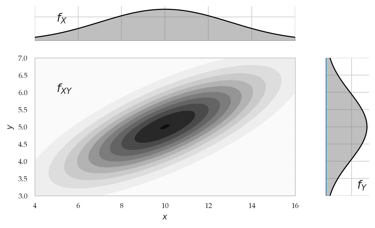
Joint probability density functions#
TODO: formulas
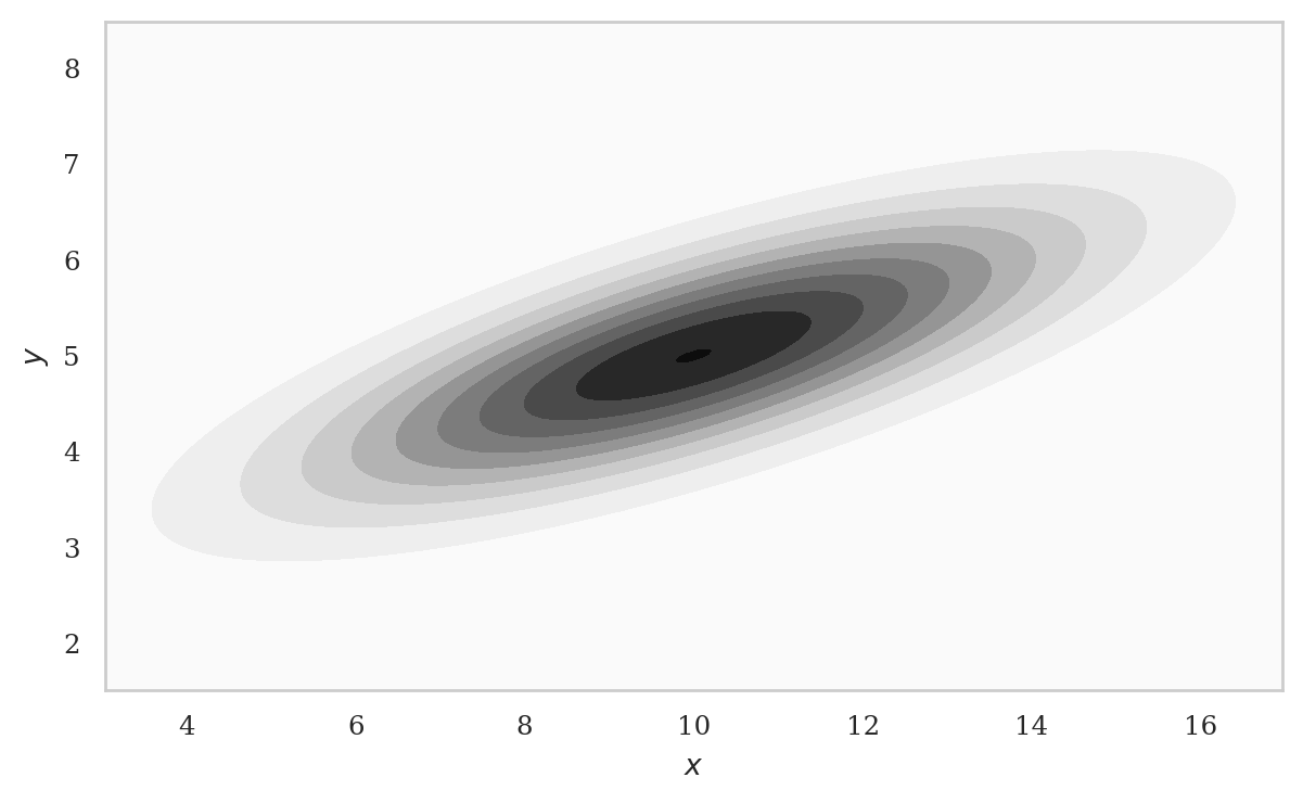
from ministats import plot_joint_pdf_contourf

xlims = [3, 17]
ylims = [1.5, 8.5]

plot_joint_pdf_contourf(rvXY, xlims=xlims, ylims=ylims);
xlims = [3, 17]
ylims = [1.5, 8.5]
event = [(10,5), (14,7)]
ax = plot_joint_pdf_contourf(rvXY, xlims=xlims, ylims=ylims, highlight=[event]);
ax.text(12, 7.3, r"$\{10 \leq X \leq 14, 5 \leq Y \leq 7\}$", ha="center");
---------------------------------------------------------------------------
TypeError                                 Traceback (most recent call last)
Cell In[11], line 4
      1 xlims = [3, 17]
      2 ylims = [1.5, 8.5]
      3 event = [(10,5), (14,7)]
----> 4 ax = plot_joint_pdf_contourf(rvXY, xlims=xlims, ylims=ylims, highlight=[event]);
      5 ax.text(12, 7.3, r"$\{10 \leq X \leq 14, 5 \leq Y \leq 7\}$", ha="center");

TypeError: plot_joint_pdf_contourf() got an unexpected keyword argument 'highlight'
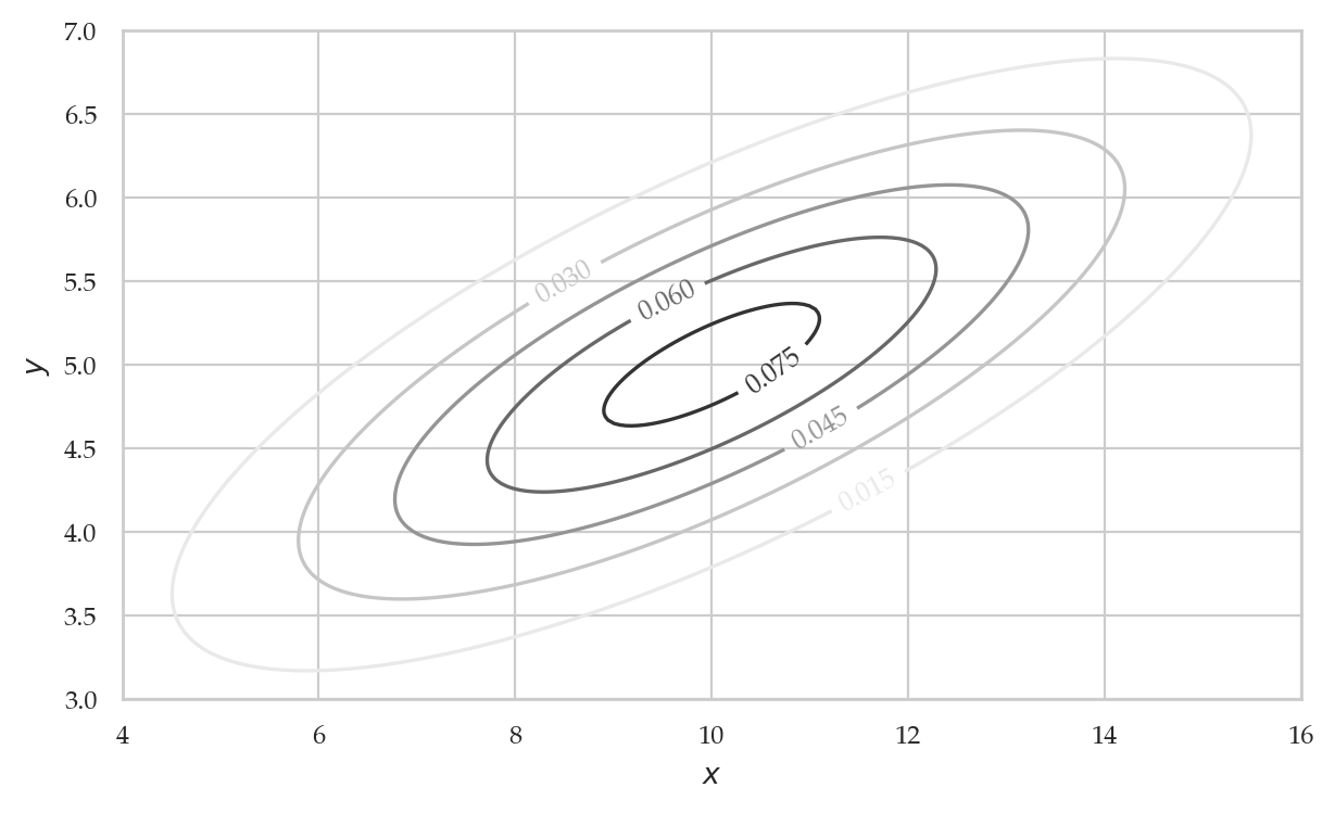
# ALT
from ministats import plot_joint_pdf_contour

xlims = [4, 16]
ylims = [3, 7]

plot_joint_pdf_contour(rvXY, xlims=xlims, ylims=ylims);
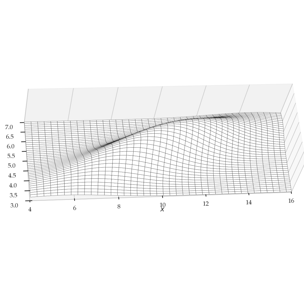
from ministats import plot_joint_pdf_surface

viewdict = dict(elev=60., azim=-110, roll=-16)
plot_joint_pdf_surface(rvXY, xlims=xlims, ylims=ylims, viewdict=viewdict);
Marginal density functions#
TODO: formulas
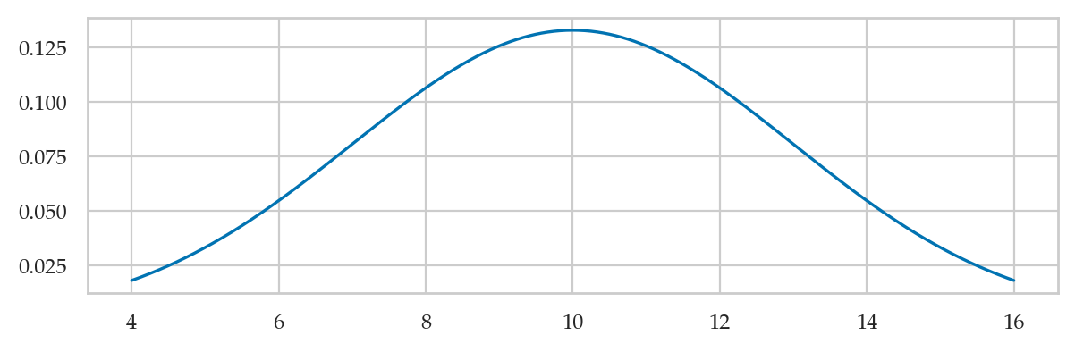
# Extract marginal f_X
rvX = rvXY.marginal(dimensions=[0])
# rvX.pdf(1), rvX.cov[0][0]
xs = np.linspace(4, 16, 1000)
fXs = rvX.pdf(xs)
sns.lineplot(x=xs, y=fXs);
# ALT. compute marginal using integration
from scipy.integrate import quad

def fX(x):
    """
    Compute the marginal density  f_X(x) = ∫ f_XY(x,y) dy.
    """
    def fXY_at_x(y):
        return rvXY.pdf([x,y])
    return quad(fXY_at_x, a=-np.inf, b=np.inf)[0]

xs = np.linspace(4, 16, 500)
fXs = [fX(x) for x in xs]
sns.lineplot(x=xs, y=fXs);

from ministats.book.figures import plot_joint_pdf_and_marginals

plot_joint_pdf_and_marginals(rvXY, xlims=xlims, ylims=ylims);
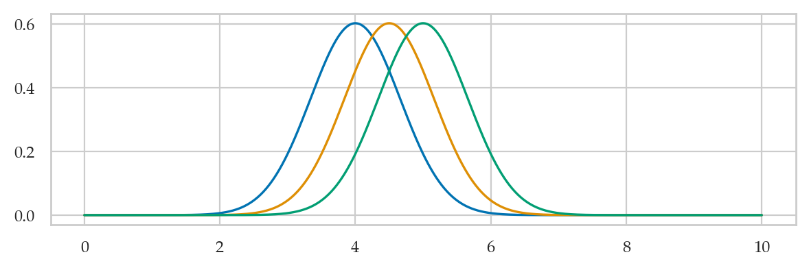
Conditional probability density functions#
# ALT
from scipy.integrate import quad

def fYgivenX(y, x_a):
    """
    Compute the conditional distribtion f_Y|X(y|x=x_a).
    """
    rvX = rvXY.marginal(dimensions=[0])
    return rvXY.pdf([x_a,y]) / rvX.pdf(x_a)

ys = np.linspace(0, 10, 1000)

fYgivenX6s = [fYgivenX(y,x_a=6) for y in ys]
sns.lineplot(x=ys, y=fYgivenX6s, c="C0")

fYgivenX8s = [fYgivenX(y,x_a=8) for y in ys]
sns.lineplot(x=ys, y=fYgivenX8s, c="C1")

fYgivenX10s = [fYgivenX(y,x_a=10) for y in ys]
sns.lineplot(x=ys, y=fYgivenX10s, c="C2");
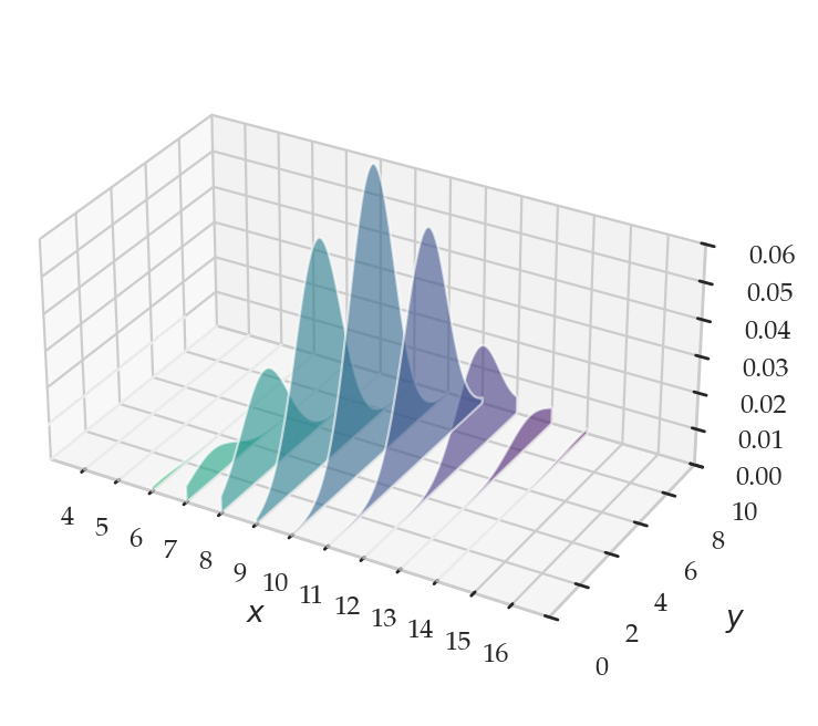
from ministats.book.figures import plot_slices_through_joint_pdf

xcuts = range(2, 15, 1)
plot_slices_through_joint_pdf(rvXY, xlims=[3,17], ylims=[0,10], xcuts=xcuts);
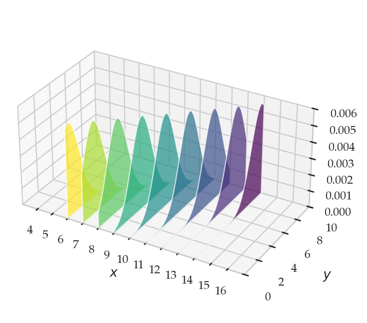
from ministats.book.figures import plot_conditional_fYgivenX

xcuts = range(6, 15, 1)
plot_conditional_fYgivenX(rvXY, xlims=[3,17], ylims=[0,10], xcuts=xcuts);
Examples#
Example: computer model for multivariate normal#
from scipy.stats import multivariate_normal

# Model parameters
muX, muY, sigmaX, sigmaY, rho = 10, 5, 3, 1, 0.75

# The mean vector
mu = [muX, muY]

# The covariance matrix
Sigma = [[         sigmaX**2,   rho*sigmaX*sigmaY ],
         [ rho*sigmaX*sigmaY,           sigmaY**2 ]]

# Multivariate normal random variable object
rvXY = multivariate_normal(mean=mu, cov=Sigma)
# Extract marginal f_X(x) = ∫ f_XY(x,y) dy
rvX = rvXY.marginal(dimensions=[0])
rvXY.cov
array([[9.  , 2.25],
       [2.25, 1.  ]])
# Extract marginal f_Y(y) = ∫f_XY(x,y)dx
rvY = rvXY.marginal(dimensions=[1])
Useful probability formulas#
Multivariable expectation#
Mean#
rvXY.mean
array([10., 5.])
Covariance#
Sigma = rvXY.cov
Sigma
array([[9.  , 2.25],
       [2.25, 1.  ]])
covXY = Sigma[0,1]
covXY
2.25
Correlation#
stdX = np.sqrt(Sigma[0,0])
stdY = np.sqrt(Sigma[1,1])

corrXY = covXY / (stdX * stdY)
corrXY
0.75
Independent, identically distributed random variabls#
TODO formulas