Section 3.6 — Statistical design and error analysis#
This notebook contains the code examples from Section 3.6 Statistical design and error analysis of the No Bullshit Guide to Statistics.
Notebook setup#
# Ensure required Python modules are installed
%pip install --quiet numpy scipy seaborn pandas ministats
[notice] A new release of pip is available: 26.1.1 -> 26.1.2
[notice] To update, run: pip install --upgrade pip
Note: you may need to restart the kernel to use updated packages.
# load Python modules
import numpy as np
import pandas as pd
import seaborn as sns
import matplotlib.pyplot as plt
# Plot helper functions
from ministats import plot_pdf
from ministats.utils import savefigure
# Figures setup
plt.clf()  # needed otherwise `sns.set_theme` doesn't work
sns.set_theme(
    context="paper",
    style="whitegrid",
    palette="colorblind",
    rc={"font.family": "serif",
        "font.serif": ["Palatino", "DejaVu Serif", "serif"],
        "figure.figsize": (10, 3)},
)
%config InlineBackend.figure_format = 'retina'
<Figure size 640x480 with 0 Axes>
# Simple float __repr__
if int(np.__version__.split(".")[0]) >= 2:
    np.set_printoptions(legacy='1.25')

# set random seed for repeatability
np.random.seed(42)
# Download datasets/ directory if necessary
from ministats import ensure_datasets
ensure_datasets()
datasets/ directory already exists.
Definitions#
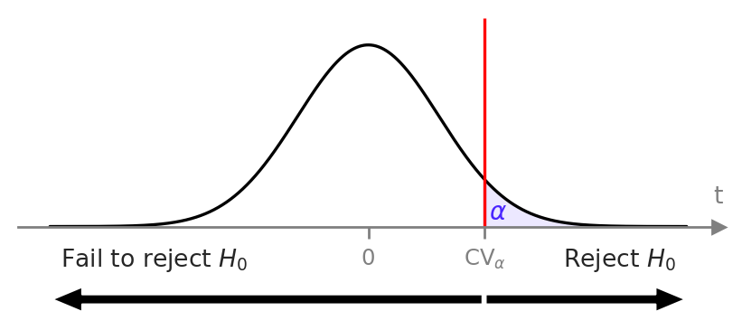
from ministats import plot_alpha_beta_errors

with sns.axes_style("ticks"), plt.rc_context({"figure.figsize":(5,1.5)}):
    plot_alpha_beta_errors(cohend=0.1, ax=None, xlims=[-3,3], n=9,
                           show_alt=False, show_concl=True,
                           alpha_offset=(0,0.014), fontsize=10)
Design params: n = 9 , alpha = 0.05 , beta = 0.910663745890349 , Delta = 0.2 , d = 0.1 , CV = 1.0965690846343148
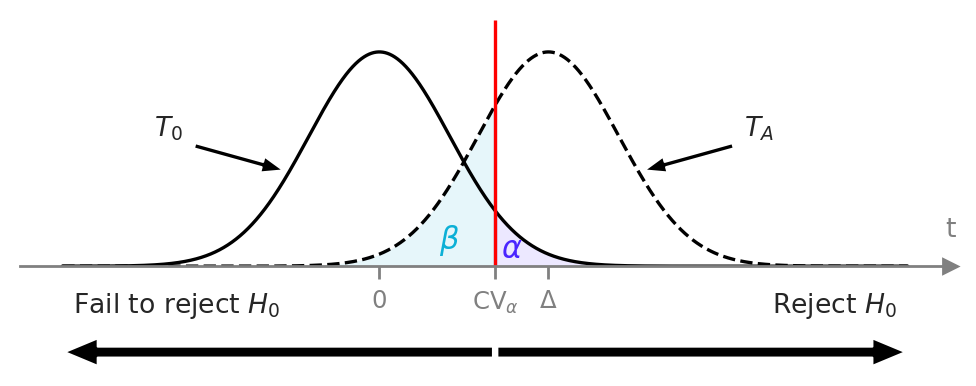
with sns.axes_style("ticks"), plt.rc_context({"figure.figsize":(6,1.6)}):
    plot_alpha_beta_errors(cohend=0.8, show_dist_labels=True,
                           show_concl=True, fontsize=11,
                           alpha_offset=(0,0.013),
                           beta_offset=(-0.06,0.02))
Design params: n = 9 , alpha = 0.05 , beta = 0.2250805806658559 , Delta = 1.6 , d = 0.8 , CV = 1.0965690846343148
Hypothesis decision rules#
Decision rule based on \(p\)-values#
# pre-data
alpha = ...   # chosen in advance

# post-data
obst = ...    # calculated from sample
rvT0 = ...    # sampling distribution under H0
pvalue = ...  # prob. of obst under rvT0

# make decision based on p-value
if pvalue <= alpha:
    decision = "Reject H0"
else:
    decision = "Fail to reject H0"
Simplified decision rule#
# pre-data
alpha = ...     # chosen in advance
rvT0 = ...      # sampling distribution under H0
CV_alpha = ...  # calculated from alpha-quantile of rvT0

# post-data
obst = ...      # calculated from sample
# make decision based on test statistic
if obst >= CV_alpha:
    decision = "Reject H0"
else:
    decision = "Fail to reject H0"
Statistical design#
# FIGURES ONLY
d_small = 0.20
d_medium = 0.57 # chosen to avoid overlap between CV and Delta
d_large = 0.80
d_vlarge = 1.3
with sns.axes_style("ticks"):
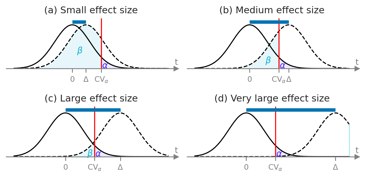
fig, ((ax1, ax2), (ax3, ax4)) = plt.subplots(2,2, figsize=(6,3))
plot_alpha_beta_errors(cohend=d_small, xlims=[-1.7,2.8], n=15, ax=ax1, fontsize=10, show_es=True,
alpha_offset=(-0.03,0.005), beta_offset=(0.1,0.2))
ax1.set_title("(a) Small effect size", fontsize=11)
plot_alpha_beta_errors(cohend=d_medium, xlims=[-1.6,2.9], n=15, ax=ax2, fontsize=10, show_es=True,
alpha_offset=(-0.03,0.005), beta_offset=(0.05,0.08))
ax2.set_title("(b) Medium effect size", fontsize=11)
plot_alpha_beta_errors(cohend=d_large, xlims=[-1.5,3], n=15, ax=ax3, fontsize=10, show_es=True,
alpha_offset=(-0.03,0.005), beta_offset=(0,0.02))
ax3.set_title("(c) Large effect size", fontsize=11)
plot_alpha_beta_errors(cohend=d_vlarge, xlims=[-1.5,3], n=15, ax=ax4, fontsize=10, show_es=True,
alpha_offset=(-0.03,0.005), beta_offset=(-0.06,0.02))
ax4.set_title("(d) Very large effect size", fontsize=11)
fig.tight_layout()
Design params: n = 15 , alpha = 0.05 , beta = 0.8079200023112518 , Delta = 0.4 , d = 0.2 , CV = 0.8493987605509224
Design params: n = 15 , alpha = 0.05 , beta = 0.28680362819561334 , Delta = 1.14 , d = 0.57 , CV = 0.8493987605509224
Design params: n = 15 , alpha = 0.05 , beta = 0.07303790512845224 , Delta = 1.6 , d = 0.8 , CV = 0.8493987605509224
Design params: n = 15 , alpha = 0.05 , beta = 0.0003494316033385532 , Delta = 2.6 , d = 1.3 , CV = 0.8493987605509224
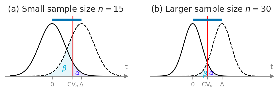
Delta = 0.6

# TODO: check this figure --> results for n=15 seem to be too good to be true...
with sns.axes_style("ticks"):
    fig, (ax1, ax2) = plt.subplots(1,2, figsize=(7,1.6))

    n1 = 15
    plot_alpha_beta_errors(cohend=Delta,  xlims=[-1.7,2.8], n=n1, ax=ax1, fontsize=10, show_es=True,
                           alpha_offset=(0.03,0.005), beta_offset=(0,0.05))
    ax1.set_title(f"(a) Small sample size $n={n1}$", fontsize=12)

    n2 = 30
    plot_alpha_beta_errors(cohend=Delta,  xlims=[-1.5,3], n=n2, ax=ax2, fontsize=10, show_es=True,
                           alpha_offset=(0.005,0), beta_offset=(0.04,0.01))
    ax2.set_title(f"(b) Larger sample size $n={n2}$", fontsize=12)
Design params: n = 15 , alpha = 0.05 , beta = 0.24858908649659617 , Delta = 1.2 , d = 0.6 , CV = 0.8493987605509224
Design params: n = 30 , alpha = 0.05 , beta = 0.0503487295055579 , Delta = 1.2 , d = 0.6 , CV = 0.6006156235170058
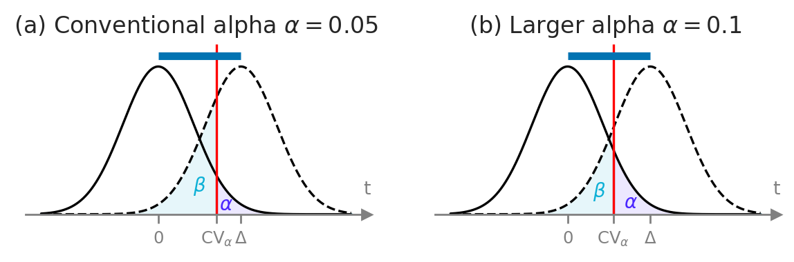
# FIGURES ONLY
Delta = 0.6

with sns.axes_style("ticks"):
    fig, (ax1, ax2) = plt.subplots(1,2, figsize=(7,1.6))

    n1 = 15
    alpha1 = 0.05
    plot_alpha_beta_errors(alpha=alpha1, cohend=Delta, xlims=[-1.7,2.8], n=15, ax=ax1, fontsize=10, show_es=True,
                           alpha_offset=(-0.02,0.005), beta_offset=(0.1,0.1))
    ax1.set_title(r"(a) Conventional alpha $\alpha=0.05$", fontsize=12)

    alpha2 = 0.1
    plot_alpha_beta_errors(alpha=alpha2, cohend=Delta, xlims=[-1.7,2.8], n=15, ax=ax2, fontsize=10, show_es=True,
                           alpha_offset=(0,0.005), beta_offset=(0.05,0.05))
    ax2.set_title(r"(b) Larger alpha $\alpha=0.1$", fontsize=12)
Design params: n = 15 , alpha = 0.05 , beta = 0.24858908649659617 , Delta = 1.2 , d = 0.6 , CV = 0.8493987605509224
Design params: n = 15 , alpha = 0.1 , beta = 0.14865057213685162 , Delta = 1.2 , d = 0.6 , CV = 0.6617903827547039
Cohen’s d standardized effect size#
The effect size \(\Delta\) we use in statistical design is usually expressed as a standardized effect size like Cohen’s \(d\), which is defined as the observed “difference” divided by a standard deviation of the theoretical model under the null hypothesis.
One-sample case#
For a one-sample test of the mean relative to a null model with mean \(\mu_0\), Cohen’s \(d\) is calculated as:
where \(s_{\mathbf{x}}\) is the sample standard deviation.
When doing statistical design, we haven’t obtained the sample \(\mathbf{x}\) yet so we don’t know what its standard deviation \(s_{\mathbf{x}}\) will be, so we have to make an educated guess of this value, which usually means using the standard deviation of the theoretical model \(\sigma_{X_0}\).
Two-sample case#
For a two-sample test for the difference between means, Cohen’s \(d\) is defined as the difference between sample means divided by the pooled standard deviation:
where the formula for the pooled variance is \(s_{p}^2 = [(n -1)s_{\mathbf{x}}^2 + (m -1)s_{\mathbf{y}}^2]/(n + m -2)\).
When doing statistical design, we don’t know the standard deviations \(s_{\mathbf{x}}\) and \(s_{\mathbf{y}}\) so we replace them with the theoretical standard deviations \(\sigma_{X_0}\) and \(\sigma_{Y_0}\) under the null hypothesis.
Recall table of reference values for Cohen’s \(d\) standardized effect sizes, suggested by Cohen in (Cohen YYYY TODO).
Cohen’s d |
Effect size |
|---|---|
0.01 |
very small |
0.20 |
small |
0.50 |
medium |
0.80 |
large |
The formulas for sample size planning and power calculations we’ll present below are based on Cohen’s \(d\).
This means you’ll have to express your guess about the effect size \(\Delta\) as \(d = \frac{\Delta}{\sigma_0}\) where \(\sigma_0\) is your best about the standard deviation of the theoretical distribution.
Note Cohen’s \(d\) is based on the standard deviations of the “raw” theoretical population, and not standard error.
Example 1: detect kombuncha volume deviation from theory#
Design Type A: choose \(\alpha=0.05\), \(\beta=0.2\), \(\Delta_{\textrm{min}} = 4\;\text{ml}\) then calculate required sample size \(n\). We’ll assume \(\sigma=10\).
alpha = 0.05
beta = 0.2
Delta_min = 4

# assumption
sigma = 10
from scipy.stats import norm
rvZ = norm(loc=0, scale=1)

z_u = rvZ.ppf(1-alpha)
z_l = rvZ.ppf(beta)

n_approx = (z_u - z_l)**2 * sigma**2 / Delta_min**2
n_approx
38.64098270012354
Using statsmodels#
To use the statsmodels sample size estimation function,
we’ll need to express the effect size \(\Delta=4\) in terms of Cohen’s \(d\).
d = Delta_min / sigma
d
0.4
from statsmodels.stats.power import TTestPower
ttp = TTestPower()
n = ttp.solve_power(effect_size=d, alpha=0.05, power=0.8,
                    alternative="larger")
n
40.02907613995644
from scipy.stats import t as tdist

rvT0 = tdist(df=n-1)
CV_alpha = rvT0.ppf(0.95)
CV_alpha
1.684844586046098
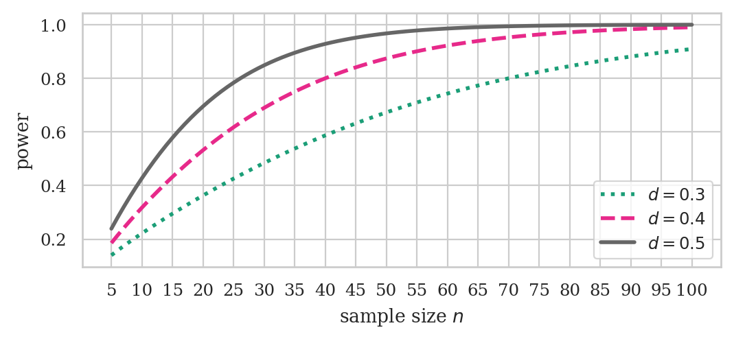
ds = np.array([0.3, 0.4, 0.5])
ns = np.arange(5, 101)
fig, ax = plt.subplots(figsize=(6,2.4))
ttp.plot_power(dep_var="nobs", ax=ax,
               effect_size=ds, nobs=ns, alpha=0.05,
               alternative="larger")
ax.set_xticks( np.arange(5,105,5) )
# ax.set_title("Power of t-test vs. sample size for different effect sizes")
ax.set_title(None)
ax.set_xlabel("sample size $n$")
ax.set_ylabel("power")
# set custom line styles
linestyles = ["dotted", "dashed", "solid"]
for line, ls in zip(ax.get_lines(), linestyles):
    line.set_linestyle(ls)
# set custom legend
labels = [f"$d={d}$" for d in ds]
ax.legend(ax.get_lines(), labels, loc="lower right");
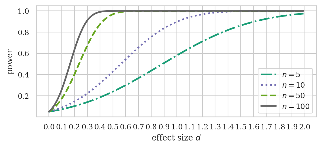
ds = np.arange(0, 2, 0.01)
ns = np.array([5, 10, 50, 100])
fig, ax = plt.subplots(figsize=(6,2.4))
ttp.plot_power(dep_var="effect size", ax=ax,
               effect_size=ds, nobs=ns, alpha=0.05,
               alternative="larger")
ax.set_xticks( np.arange(0, 2+0.1, 0.1) )
# ax.set_title("Power of t-test vs. effect size for different sample sizes")
ax.set_title(None)
ax.set_xlabel("effect size $d$")
ax.set_ylabel("power")

# set custom line styles
linestyles = ["dashdot", "dotted", "dashed", "solid"]
for line, ls in zip(ax.get_lines(), linestyles):
    line.set_linestyle(ls)
# set custom legend
labels = [f"$n={n}$" for n in ns]
ax.legend(ax.get_lines(), labels);
Data collection#
kombuchapop = pd.read_csv("datasets/kombuchapop.csv")
batch55pop = kombuchapop[kombuchapop["batch"]==55]
kpop55 = batch55pop["volume"]
We can select a random sample of size \(n=41\) from the populaiton kpop55
by calling the .sample method.
np.random.seed(71)
n = 41  # rounding up
ksample55 = kpop55.sample(n)
len(ksample55)
41
# Uncomment to see the observed sample
# ksample55.values
# Observed sample mean
np.mean(ksample55)
1001.6541463414634
# Observed effect size from Batch 55
Delta_hat = np.mean(ksample55) - 1000
Delta_hat
1.6541463414633881
Statistical analysis on the sample from Batch 55#
CV_alpha # = tdist(df=n-1).ppf(0.95)
1.684844586046098
kbar55 = ksample55.mean()
sehat55 =  ksample55.std() / np.sqrt(n)

t55 = (kbar55 - 1000) / sehat55
t55
1.1024261132512938
We can now apply the simplified decision rule
that compares the test statistic t55
to the cutoff value CV_alpha.
if t55 >= CV_alpha:
    decision = "Reject H0"
else:
    decision = "Fail to reject H0"
decision
'Fail to reject H0'
Alternatively,
we can make the decision whether to reject \(H_0\) or not
using the “old” decision rule that compares the
\(p\)-value to the cutoff \(\alpha=0.05\).
We can compute the p-value from ttest_mean function we defined
in Section 3.4, see 34_analytical_approx.ipynb.
from ministats import ttest_mean
pvalue55 = ttest_mean(ksample55, mu0=1000)
print("p-value =", pvalue55)
if pvalue55 <= 0.05:
    decision = "Reject H0"
else:
    decision = "Fail to reject H0"
decision
p-value = 0.276865468844746
'Fail to reject H0'
# ALT2. Use the p-value form a direct simulation test
from ministats import simulation_test_mean
simulation_test_mean(ksample55, mu0=1000, sigma0=10)
0.2917
Example 2: comparison of East vs. West electricity prices#
eprices = pd.read_csv("datasets/eprices.csv")
eprices.groupby("loc").describe()
| price | ||||||||
|---|---|---|---|---|---|---|---|---|
| count | mean | std | min | 25% | 50% | 75% | max | |
| loc | ||||||||
| East | 9.0 | 6.155556 | 0.877655 | 4.8 | 5.5 | 6.3 | 6.5 | 7.7 |
| West | 9.0 | 9.155556 | 1.562139 | 6.8 | 8.3 | 8.6 | 10.0 | 11.8 |
Need a guess the effect size, which we’ll express in terms of Cohen’s \(d\). We choose \(d=1\), which corresponds to a difference of one cent \(\Delta_{\text{min}} = 1\), assuming the standard deviation of the prices is around \(\sigma=1\).
cohend2_min = 1
Solving for a desired power#
The function solve_power takes as argument the chosen level of power,
and two of the three other design parameters alpha, nobs1, and effect_size,
and calculates the value of the third parameter required to achieve the chosen level of power \(=(1-\beta)\).
from statsmodels.stats.power import TTestIndPower
ttindp = TTestIndPower()

# power of two-sample t-test assuming cohend2_min and n=m=9
ttindp.power(effect_size=cohend2_min, nobs1=9,
             alpha=0.05, alternative="two-sided")
0.5133625331067571
The Type II error rate \(\beta\) of this test is
1 - 0.5133625331068463
0.4866374668931537
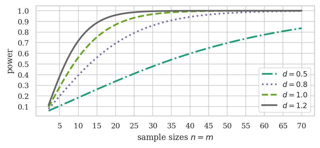
ds = np.array([0.5, 0.8, 1.0, 1.2])
ns = np.arange(2, 71)
fig, ax = plt.subplots(figsize=(6,2.4))
ttindp.plot_power(dep_var="nobs", ax=ax,
                  effect_size=ds, nobs=ns, alpha=0.05,
                  alternative="two-sided")
ax.set_xticks( np.arange(5,75,5) )
# ax.set_title("Power of two-sample t-test vs. sample size $n=m$ for different effect sizes")
ax.set_title(None)
ax.set_xlabel("sample sizes $n=m$")
ax.set_yticks([0.1, 0.2,0.3,0.4,0.5,0.6,0.7,0.8,0.9,1.0])
ax.set_ylabel("power")

# set custom line styles
linestyles = ["dashdot", "dotted", "dashed", "solid"]
for line, ls in zip(ax.get_lines(), linestyles):
    line.set_linestyle(ls)
# set custom legend
labels = [f"$d={d}$" for d in ds]
ax.legend(ax.get_lines(), labels);
If Bob wants to achieve 80% power for future price comparison tests, he needs to collect samples of size \(n=1\) or larger.
ttindp.solve_power(effect_size=cohend2_min, power=0.8, alpha=0.05,
                   alternative="two-sided")
16.714722446954024
Calculate minimum effect size#
# minimum effect size to achieve 80% power when n=m=9
ttindp.solve_power(alpha=0.05, power=0.8, nobs1=9,
                   alternative="two-sided")
1.4069246523451708
(optional) Calculate sample size needed to achieve 0.8 power#
# minimum sample size required to achieve 80% power when effect size is d=1
ttindp.solve_power(effect_size=1.0, alpha=0.05, power=0.8,
                   alternative="two-sided")
16.714722446954024
Alternative calculation methods#
Using G*Power#
TODO: add sceenshots
Using pingouin#
import pingouin as pg
Sample size for the one-sample \(t\)-test#
pg.power_ttest(alpha=0.05, power=0.8, d=0.4,
               contrast="one-sample", alternative="greater")
40.02907622585533
We can also verify that \(n=41\) produces a test with \(80\%\) power.
pg.power_ttest(alpha=0.05, n=41, d=0.4,
               contrast="one-sample", alternative="greater")
0.8085822361693651
Power of Bob’s two-sample \(t\)-test#
# power of two-sample t-test assuming d=1 and n=m=9
pg.power_ttest(alpha=0.05, n=9, d=1,
               contrast="two-samples", alternative="two-sided")
0.5133625331067571
Explanations#
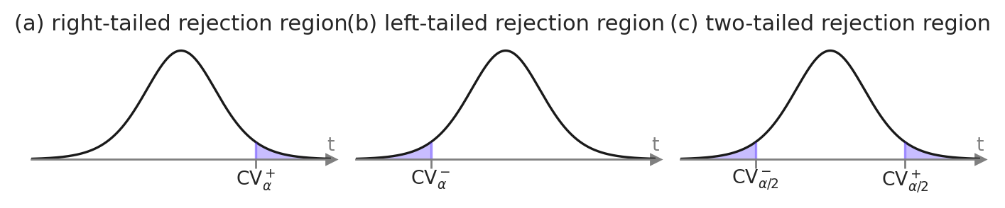
One-sided and two-sided rejection regions#
from scipy.stats import t as tdist
rvT0 = tdist(df=9)

alpha = 0.05

# right-tailed rejection region
rvT0.ppf(alpha)
-1.8331129326562376
# left-tailed rejection region
rvT0.ppf(1-alpha)
1.833112932656237
# two-sided rejection region
rvT0.ppf(alpha/2), rvT0.ppf(1 - alpha/2)
(-2.2621571627982053, 2.262157162798205)
from ministats.book.figures import plot_panel_rejection_regions

plot_panel_rejection_regions();
Derivation of the sample size planning formula#
MAYBE show math steps
Discussion#
A conceptual amalgam of two ideas#
Steps of the Neyman—Pearson hypothesis test#
Calculate the cutoff value \(\text{CV}_{\alpha}\).
Calculate the test statistic \(t_{55}\) from the sample \(\mathbf{k}_{55}\).
Apply the simplified decision rule that compares the test statistic to the cutoff value.
# 1. Calculate the critical value
from scipy.stats import t as tdist
rvT0 = tdist(df=n-1)
CV_alpha = rvT0.ppf(0.95)
CV_alpha
1.683851013335652
# 2. Calculate the test statistic
n = len(ksample55)
kbar55 = ksample55.mean()
sehat55 =  ksample55.std() / np.sqrt(n)
t55 = (kbar55 - 1000) / sehat55
t55
1.1024261132512938
# 3. Compare the test-statistic to the critical value
if t55 >= CV_alpha:
    decision = "Reject H0"
else:
    decision = "Fail to reject H0"
decision
'Fail to reject H0'
Steps of the Fisherian hypothesis test#
Calculate the test statistic \(t_{55}\).
Calculate the \(p\)-value of the statistic from the sampling distribution under \(H_0\).
Make a decision whether to reject \(H_0\) by comparing the \(p\)-value to the cutoff \(\alpha=0.05\).
# 1. Calculate the test statistic
n = len(ksample55)
kbar55 = ksample55.mean()
sehat55 =  ksample55.std() / np.sqrt(n)
t55 = (kbar55 - 1000) / sehat55
t55
1.1024261132512938
# 2. Calculate the $p$-value
from scipy.stats import t as tdist
rvT0 = tdist(df=n-1)
pvalue55 = 1 - rvT0.cdf(t55)   # right-tailed p-value
pvalue55
0.13843273442237303
By the way,
we can also obtain the \(p\)-value
by calling the helper function ttest_mean
that we defined in Section 3.4, see 34_analytical_approx.ipynb.
from ministats import ttest_mean
ttest_mean(ksample55, mu0=1000, alt="greater")
0.13843273442237303
# 3. Compare the p-value to the cutoff alpha
if pvalue55 <= 0.05:
    decision = "Reject H0"
else:
    decision = "Fail to reject H0"
decision
'Fail to reject H0'
We see the results of the Neyman–Pearson and Fisherian decision rules are the same. Indeed, we’ll always come to the same decision, whether we use criterion \(p < \alpha\) in the space of \(p\)-values, or the \(t_{55} \geq \text{CV}_{\alpha}\) in the space of \(t\)-values.
Post-hoc power analysis#
# Observed effect size from Batch 55
Delta_hat = np.mean(ksample55) - 1000
Delta_hat
1.6541463414633881
# Observed effect size as Cohen's d
d_hat = Delta_hat / 10
d_hat
0.1654146341463388
The post-hoc power for the test we performed in Example~1 is:
from statsmodels.stats.power import TTestPower
ttp = TTestPower()
ttp.power(alpha=0.05, nobs=41, effect_size=d_hat, alternative="larger")
0.2730623700889534
It’s not clear what this power means…
Unique value proposition of hypothesis testing#
Exercises#
Exercise {exercise:sensitivity-of-one-sample-t-test-n-10}#
from statsmodels.stats.power import TTestPower
ttp = TTestPower()
ttp.solve_power(alpha=0.05, power=0.8, nobs=10, alternative="larger")
0.8528391375729825
Exercise {exercise:power-of-two-sample-t-test-n-17}#
from statsmodels.stats.power import TTestIndPower
ttindp = TTestIndPower()
ttindp.power(alpha=0.05, nobs1=17, effect_size=1, alternative="two-sided")
0.8070367151472196