Section 2.7 — Simulation and empirical distributions#
This notebook contains the code examples from Section 2.7 Simulation and empirical distributions of the No Bullshit Guide to Statistics.
Notebook setup#
# Ensure required Python modules are installed
%pip install --quiet numpy scipy seaborn ministats
Note: you may need to restart the kernel to use updated packages.
# Load Python modules
import numpy as np
import pandas as pd
import random
import seaborn as sns
import matplotlib.pyplot as plt
# Figures setup
plt.clf()  # needed otherwise `sns.set_theme` doesn't work
sns.set_theme(
    context="paper",
    style="whitegrid",
    palette="colorblind",
    rc={"font.family": "serif",
        "font.serif": ["Palatino", "DejaVu Serif", "serif"],
        "figure.figsize": (7,2)},
)
%config InlineBackend.figure_format = "retina"
<Figure size 640x480 with 0 Axes>
# Simple float __repr__
import numpy as np
if int(np.__version__.split(".")[0]) >= 2:
    np.set_printoptions(legacy='1.25')
Why simulate?#
Running simulations of random variables is super useful:
Simplified probability calculations: no need for complicated integrals, since we can replace any calculation you might want to do with the distribution \(f_X\) with an equivalent calculation on the list of observations \([x_1,x_2,\ldots,x_N]\)
Visualize probability theory results: using simulations based on random observations \([x_1, x_2, x_3, \ldots, x_N]\), we can visualize these theoretical results to gain hands-on intuition and experience with them.
Verify that statistics procedures work: we can use simulation to experimentally verify the performance of the statistical procedure. Does a procedure really work correctly 95% of the time? Simulate 1000 datasets and count the proportion of times when the procedure worked correctly.
In the remainder of this section, we’ll learn how to use the list of observations \([x_1,x_2,\ldots,x_N]\) as an alternative to the math calculations with the random variable \(X\), including visualizations and various probabilities.
Observations from random variables#
Generating lists of random observations#
from scipy.stats import expon

lam = 0.2
rvE = expon(loc=0, scale=1/lam)
np.random.seed(44)

N = 1000  # number of observations to generate
es = rvE.rvs(N)
es[0:7].round(3)
array([9.004, 0.554, 6.825, 2.235, 2.226, 4.698, 2.503])
Visualizing probability distribution#
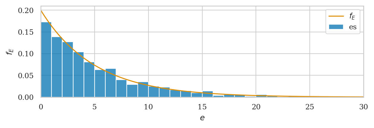
# Plot a histogram of the simulated data
ax = sns.histplot(es, bins=range(0,31), stat="density", label="es");

# Plot the PDF of rvE
from ministats import plot_pdf
plot_pdf(rvE, rv_name="E", color="C1", ax=ax, label="$f_E$");
ax.set_xlim([0,30]);
Calculate the mean and variance#
import numpy as np
np.mean(es), rvE.mean()
(5.119377169180479, 5.0)
np.var(es), rvE.var()
(25.12355642871208, 25.0)
np.std(es), rvE.std()
(5.012340414288726, 5.0)
Calculate probabilities#
len([e for e in es if e >= 7]) / len(es)
0.247
from scipy.integrate import quad
quad(rvE.pdf, 7, np.inf)[0]
0.2465969639416065
1 - rvE.cdf(7)
0.24659696394160646
Compute expectations#
def fatigue(e):
    return 10 / (1 + e)

np.mean([fatigue(e) for e in es])
2.894485288770725
rvE.expect(fatigue)
2.986697493864491
Empirical distributions#
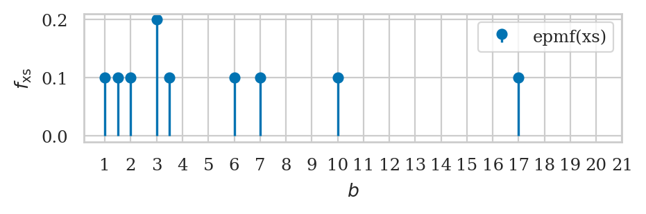
Empirical probability mass function#
xs = [1, 1.5, 2, 3, 3, 3.5, 6, 7, 10, 17]
from ministats import plot_epmf

plot_epmf(xs, name="xs");
Generating bootstrap observations#
Suppose we want to simulate new random observations form \(f_E\),
but for some reason we don’t have access to the method rvE.rvs anymore.
np.random.seed(52)

xs_boot = np.random.choice(xs, 5, replace=True)
xs_boot
array([3.5, 7. , 6. , 7. , 1. ])
[x_boot in xs for x_boot in xs_boot]
[True, True, True, True, True]
list(xs_boot).count(7)
2
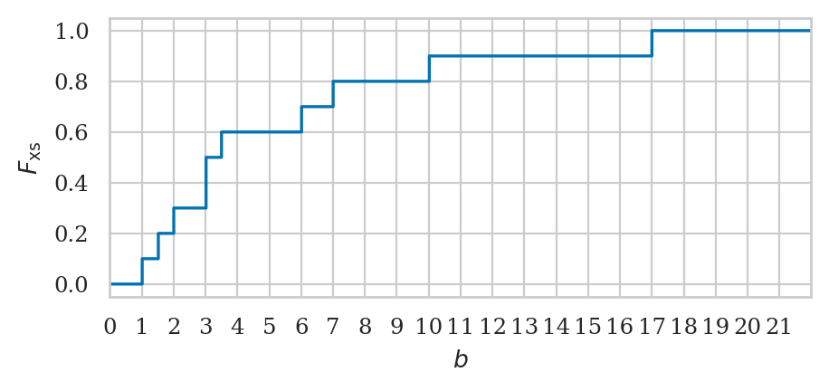
Empirical cumulative distribution function#
Let’s write a function that compute the value empirical cumulative distribution (empirical CDF)
of the sample data. The function takes two inputs: data the sample of observations,
and b, the value where we want to evaluate the function.
def ecdf(data, b):
    sorted_data = np.sort(data)
    count = sum(sorted_data <= b)  # num. of obs. <= b
    return count / len(data)       # proportion of total
Note the sorting step is not strictly necessary,
but it guarantees the sdata is a NymPy array object which allows the comparison to work.
ecdf(xs, 5)
0.6
ecdf(xs, 10)
0.9
import seaborn as sns
sns.ecdfplot(x=xs);
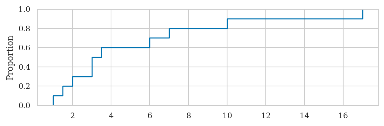
# ALT. use the `plot_ecdf` function from `ministats`
from ministats import plot_ecdf
ax = plot_ecdf(xs, name="xs")
Inverse of the empirical cumulative distribution function#
def inv_ecdf(data, q):
    return np.quantile(data, q, method="inverted_cdf")

# TEST inv_ecdf
# K = 1000
# qs = np.linspace(0, 1, K)
# qs2 = np.ndarray(K)
# for i, q in enumerate(qs):
#     x = inv_ecdf(es, q)
#     q2 = ecdf(es, x)
#     qs2[i] = q2
# sns.histplot(qs2 - qs)
TODO: explain inverse empirical CDF
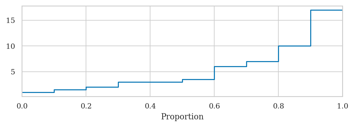
sns.ecdfplot(y=xs);
Random variable generation from scratch#
Uniform random variable primitive#
import numpy as np
np.random.seed(41)
np.random.rand()
0.25092362374494015
np.random.seed(42)
np.random.rand()
0.3745401188473625
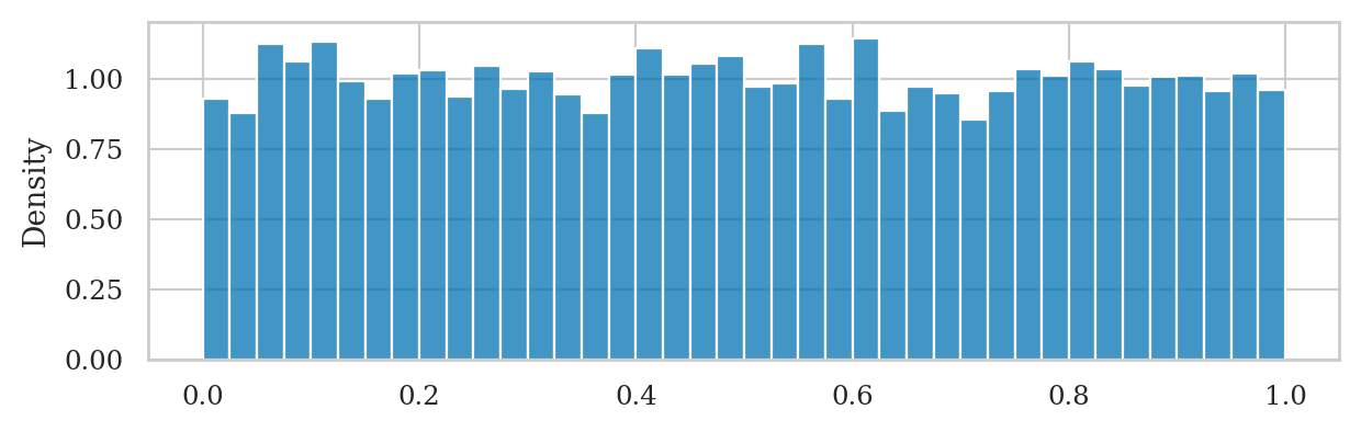
np.random.seed(45)

us = np.random.rand(8000)
sns.histplot(us, bins=40, stat="density");
Continuous random variable generation#
See the book or explanations of the the invers-CDF trick.
Generating exponentially distributed observations#
def gen_e(lam):
    u = np.random.rand()
    e = -1 * np.log(1-u) / lam
    return e
Where lam is the \(\lambda\) (lambda) parameter chosen for exponential model family.
np.random.seed(26)

N = 200  # number of observations to generate
es2 = [gen_e(lam=0.2) for i in range(N)]
es2[0:5] # first five observations
[1.8403766434262139,
 3.663511132756237,
 7.311508774831116,
 7.784719180427214,
 10.222768798178041]
# [e.round(3) for e in es2[0:5]] # first five observations
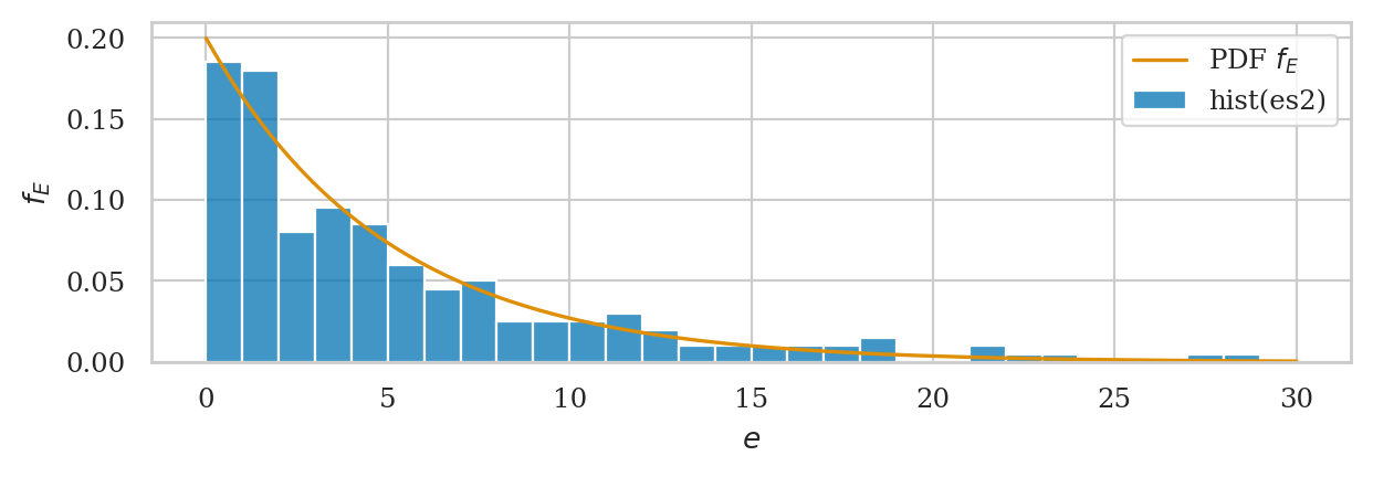
# Plot a histogram of data in `es2`
ax = sns.histplot(es2, bins=range(30), stat="density", label="hist(es2)")

# Plot the PDF of rvE
from ministats import plot_pdf
plot_pdf(rvE, rv_name="E", xlims=[0,30], color="C1", ax=ax, label="PDF $f_E$");
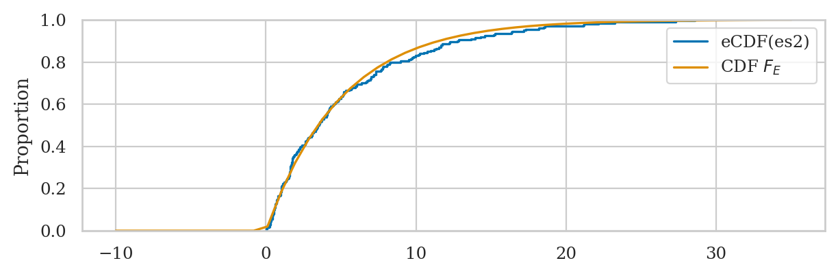
# Plot the empirical CDF of es2
ax = sns.ecdfplot(es2, label="eCDF(es2)")

# Plot the CDF of rvE on the same axis
from ministats import plot_cdf
plot_cdf(rvE, rv_name="E", xlims=[0,30], ax=ax, color="C1", label="CDF $F_E$")
ax.set_xlabel(None)
ax.set_xticks(range(0,31,5));
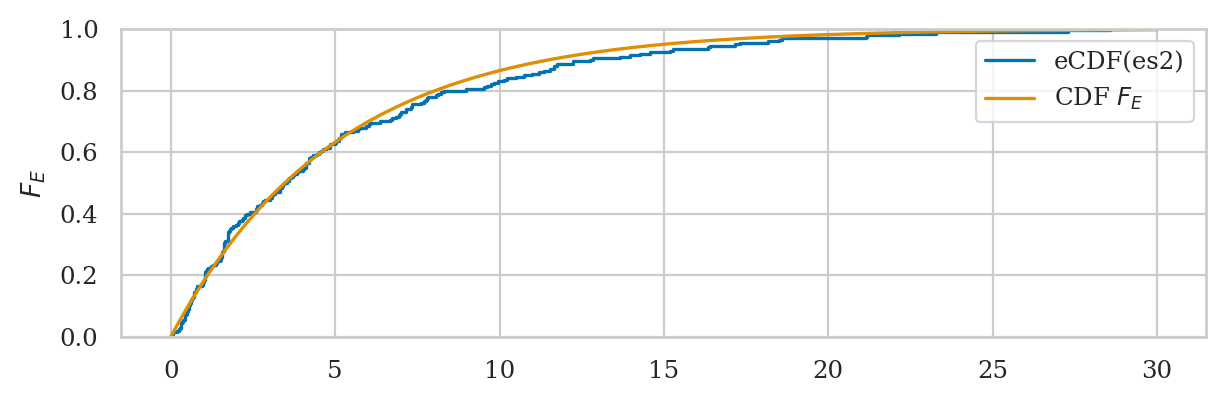
We’ll develop various way to analyze this “goodness of fit” between the sample es data we generated
and the theoretical model \(f_E\) in the remainder of this notebook.
Measuring data-model fit#
Want to measure if es comes from \(\textrm{Expon}(\lambda=0.2)\).
Here are the first five values we simulated:
es2[0:5]
[1.8403766434262139,
 3.663511132756237,
 7.311508774831116,
 7.784719180427214,
 10.222768798178041]
Visual comparison between data and model distributions#
from scipy.stats import expon
lam = 0.2
rvE = expon(0, 1/lam)
Here is the code for visual comparison of es2 and the theoretical model rvE \(=\mathrm{Expon}(\lambda=0.2)\), based on the probability density and cumulative probability distributions.
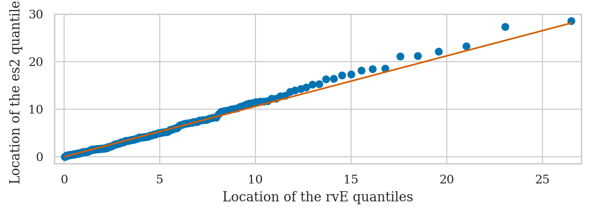
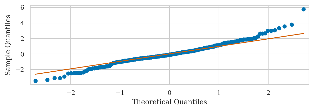
Using Q-Q plots to compare quantiles#
The quantile-quantile plot qq_plot(data, dist)
is used to compare the positions of the quantiles of the dataset data
against the quantiles of the theoretical distribution dist,
which is an instance of one of the probability models in scipy.stats.
Exponential sample vs. true exponential model#
from statsmodels.graphics.api import qqplot
fig = qqplot(np.array(es2), dist=rvE, line="q")
fig.axes[0].set_xlabel("Location of the rvE quantiles")
fig.axes[0].set_ylabel("Location of the es2 quantiles");
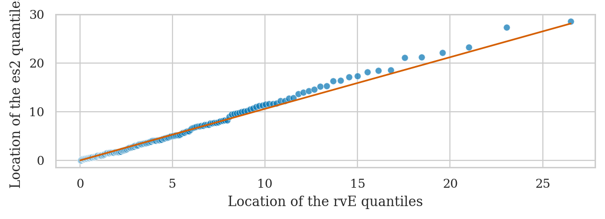
Another way to generate a Q-Q plot is to use
the function qqplot defined in the the statsmodels package.
# ALT. use the helper function `qq_plot` from `ministats`
from ministats import qq_plot
ax = qq_plot(es2, dist=rvE)
ax.set_xlabel("Location of the rvE quantiles")
ax.set_ylabel("Location of the es2 quantiles");
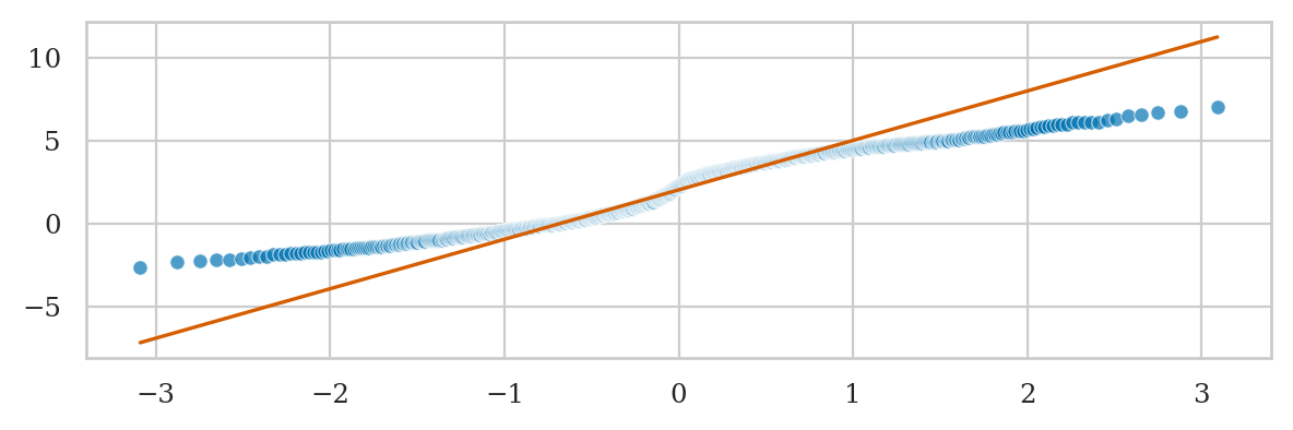
Exponential data vs. standard normal#
from scipy.stats import norm
qqplot(np.array(es2), dist=norm(0,1), line="q");
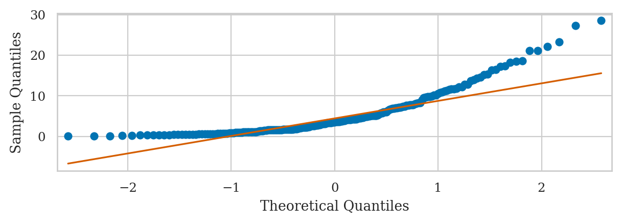
Note the lowest quantiles don’t match (exponential data limited to zero), and the high quantiles don’t match either (exponential data has a long tail).
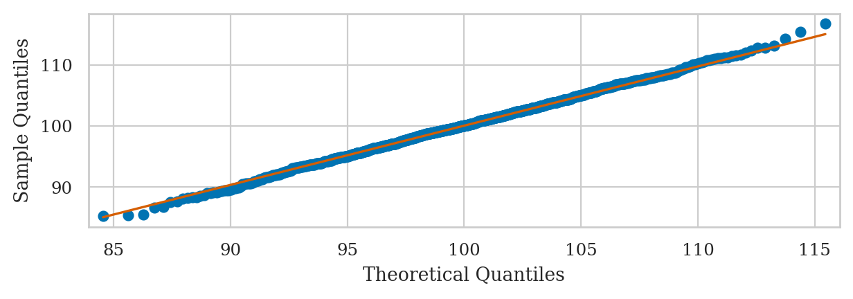
Normal data vs. standard normal#
Here is an example of a Q-Q plot with very good fit.
rvN = norm(100, 5)
ns = rvN.rvs(1000)
qqplot(ns, dist=rvN, line="q");
Student’s t-data vs. standard normal#
from scipy.stats import t as tdist
np.random.seed(46)
rvT = tdist(df=5)
ts = rvT.rvs(300)
qqplot(ts, dist=norm(0,1), line="q");
Bimodal data vs. standard normal (BONUS EXAMPLE)#
from ministats.probs import MixtureModel

np.random.seed(47)
rvBN = MixtureModel([norm(0,1), norm(4, 1)], weights=[0.5,0.5])
bns = rvBN.rvs(1000)
qq_plot(bns, dist=norm(0,1));
Comparing moments#
A simple way to measure how well the data sample \(\mathbf{x} = (x_1, x_2, \ldots , x_n)\) fits the probability model \(f_X\) is to check if the data distribution and the probability distribution have the same moments.
In order to easily be able to calculate the moments of the data samples,
we’ll convert es into a pandas series object,
which has all the necessary methods.
es2_series = pd.Series(es2)
es2_series.mean(), rvE.mean()
(5.3330881197327535, 5.0)
es2_series.var(), rvE.var()
(30.45191637582025, 25.0)
Let’s now compare the skew of dataset and the skew of the distribution:
es2_series.skew(), rvE.stats("s")
(1.711852367068079, 2.0)
Finally, let’s compare the kurtosis of dataset and the kurtosis of the distribution.
es2_series.kurt(), rvE.stats("k")
(3.0431185936008607, 6.0)
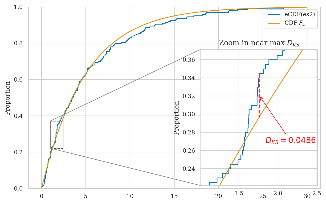
Kolmogorov–Smirnov distance#
from scipy.stats import ks_1samp
Let’s jump right ahead and compute the KS distance for the data and distribution of interest.
ks_1samp(es2, rvE.cdf).statistic
0.048609282602185055
sns.ecdfplot(es2, label="eCDF(es2)")
bs = np.linspace(-10,35)
sns.lineplot(x=bs, y=rvE.cdf(bs), label="CDF $F_E$");
from ministats.book.figures import plot_ks_dist_with_inset

plot_ks_dist_with_inset(es2, rvE, label_sample="eCDF(es2)", label_rv="CDF $F_E$");
Discussion#
Seeding random number generators#
Every time you run the following two cells, you’ll get different numbers.
from scipy.stats import norm
rvZ = norm(0,1)
rvZ.rvs(3)
array([-1.29926108, 1.10740701, 1.66512925])
rvZ.rvs(3)
array([ 0.82613809, -0.93630083, -1.2185572 ])
We can set random seed for repeatability.
import numpy as np
np.random.seed(46)
rvZ.rvs(3)
array([0.58487584, 1.23119574, 0.82190026])
np.random.seed(46)
rvZ.rvs(3)
array([0.58487584, 1.23119574, 0.82190026])