Welch’s two-sample \(t\)-test#
The goal of Welch’s two-sample \(t\)-test to check if the means two unknown population \(X \sim \mathcal{N}(\mu_X, \sigma_X)\) and \(Y \sim \mathcal{N}(\mu_Y, \sigma_Y)\) are the same or different.
For statistical design considerations related to two-sample tests,
see the notebook statistical_design.ipynb.
import matplotlib.pyplot as plt
import numpy as np
import seaborn as sns
import pandas as pd
%matplotlib inline
%config InlineBackend.figure_format = 'retina'
\(\def\stderr#1{\mathbf{se}_{#1}}\) \(\def\stderrhat#1{\widehat{\mathbf{se}}_{#1}}\) \(\newcommand{\Mean}{\textbf{Mean}}\) \(\newcommand{\Var}{\textbf{Var}}\) \(\newcommand{\Std}{\textbf{Std}}\) \(\newcommand{\Freq}{\textbf{Freq}}\) \(\newcommand{\RelFreq}{\textbf{RelFreq}}\) \(\newcommand{\DMeans}{\textbf{DMeans}}\) \(\newcommand{\Prop}{\textbf{Prop}}\) \(\newcommand{\DProps}{\textbf{DProps}}\)
Data#
Two samples of numerical observations \(\mathbf{x}=[x_1, x_2, \ldots, x_n]\) and \(\mathbf{y}=[y_1, y_2,\ldots, y_m]\) from independent populations.
Assumptions#
We assume the unknown populations are normally distributed \(\textbf{(NORM)}\), or the sample is large enough \(\textbf{(LARGEn)}\), so that the sampling distributions of the means in the two populations will be approximately normally distributed:
where \(\sigma_X\) and \(\sigma_Y\) are the standard deviations of the unknown populations.
Hypotheses#
\(H_0: \mu_X = \mu_Y\) and \(H_A: \mu_X \neq \mu_Y\).
Estimates#
Compute the sample means \(\overline{\mathbf{x}} = \Mean(\mathbf{x}) = \frac{1}{n}\sum_{i=1}^n x_i\), \(\overline{\mathbf{y}} = \Mean(\mathbf{y}) = \frac{1}{m}\sum_{i=1}^m y_i\), and the observed difference between means \(\hat{d} = \DMeans(\mathbf{x}, \mathbf{y}) = \overline{\mathbf{x}} - \overline{\mathbf{y}}\).
We need to also compute the standard deviations \(s_{\mathbf{x}} = \Std(\mathbf{x}) = \sqrt{ \frac{1}{n-1}\sum_{i=1}^n (x_i-\overline{\mathbf{x}})^2 }\) and \(s_{\mathbf{y}} = \Std(\mathbf{y}) = \sqrt{ \frac{1}{m-1}\sum_{i=1}^m (y_i-\overline{\mathbf{y}})^2 }\), which are estimates for the unknown population standard deviations \(\sigma_X\) and \(\sigma_Y\).
Formulas#
The estimated standard error of the difference-between-means estimator is
where \(s_{\mathbf{x}}\) and \(s_{\mathbf{y}}\) are the sample standard deviations.
The Welch–Satterthwaite formula for the degrees of freedom parameter \(\nu_d\) is
In Python, we can calculate \(\nu_d\) by calling the helper function calcdf:
\(\nu_d = \tt{calcdf}(s_{\mathbf{x}}, n, s_{\mathbf{y}}, m)\).
Test statistic#
Compute the \(t\)-statistic \(t = \frac{\hat{d} - 0}{ \stderrhat{\hat{d}} }\).
Sampling distribution#
Student’s \(t\)-distribution with \(\nu_d\) degrees of freedom,
where the degrees of freedom parameter is computed using
the helper function calcdf:
\(\nu_d = \tt{calcdf}(s_{\mathbf{x}}, n, s_{\mathbf{y}}, m)\),
which implements the Welch–Satterthwaite formula.
P-value calculation#
To obtain the \(p\)-value, we first compute the observed \(t\)-statistic, then calculate the tail probabilities in the two tails of the standard normal distribution \(T_0 \sim \mathcal{T}(\nu_d)\).
from ministats import ttest_dmeans
from scipy.stats import ttest_ind
Let’s look at the source code of the function ttest_dmeans,
which performs the steps of the two-sample t-test.
import numpy as np
from scipy.stats import t as tdist
from ministats import mean, std, calcdf, tailprobs

def ttest_dmeans(xsample, ysample, alt="two-sided"):
    """
    T-test to detect difference between two populations means
    based on the difference between sample means.
    """
    # Calculate the observed difference between means
    obsdhat = mean(xsample) - mean(ysample)

    # Calculate the sample sizes and the stds
    n, m = len(xsample), len(ysample)
    sx, sy = std(xsample), std(ysample)

    # Calculate the standard error, the degrees of
    # freedom, the null model, and the t-statistic
    seD = np.sqrt(sx**2/n + sy**2/m)
    obst = (obsdhat - 0) / seD
    dfD = calcdf(sx, n, sy, m)
    rvT0 = tdist(df=dfD)

    # Calculate the p-value from the t-distribution
    pvalue = tailprobs(rvT0, obst, alt=alt)
    return pvalue
See Section 3.5 in the No Bullshit Guide to Statistics for the detailed explanation of these steps. You can also check out the section Analytical approximation methods in the notebook notebooks/35_two_sample_tests.ipynb.
To perform the two-sample \(t\)-test on the samples xs and ys,
we call ttest_dmeans(xs, ys) or ttest_ind(xs, ys, equal_var=False),
as we’ll show in the Examples section below.
Effect size estimates#
from ministats import ci_dmeans
import numpy as np
from scipy.stats import t as tdist
from ministats import calcdf

def ci_dmeans(xsample, ysample, alpha=0.1):
    """
    Compute confidence interval for the difference between population means.
    """
    stdX, n = np.std(xsample, ddof=1), len(xsample)
    stdY, m = np.std(ysample, ddof=1), len(ysample)
    dhat = np.mean(xsample) - np.mean(ysample)
    seD = np.sqrt(stdX**2/n + stdY**2/m)
    dfD = calcdf(stdX, n, stdY, m)
    t_l = tdist(df=dfD).ppf(alpha/2)
    t_u = tdist(df=dfD).ppf(1-alpha/2)
    return [dhat + t_l*seD, dhat + t_u*seD]
TODO: narrate code
To use the function …
Examples#
Let’s start by generating some samples from the following three populations for use in the examples we present below.
Note populations \(B\) and \(C\) are identical.
We’ll now generate a samples of size \(n=20\) from each of these populaitons
and store them in a Pandas data frame called data.
from scipy.stats import norm

np.random.seed(42)

n = 20   # sample size

# Sample A: size = 20, population = N(104,3)
avals = norm(104,3).rvs(n)
dataA = pd.DataFrame({"pop":["A"]*n, "val":avals})

# Sample B: size=20, population = N(100,5)
bvals = norm(100,5).rvs(n)
dataB = pd.DataFrame({"pop":["B"]*n, "val":bvals})

# Sample C: size=20, same population as Sample B
cvals = norm(100,5).rvs(n)
dataC = pd.DataFrame({"pop":["C"]*n, "val":cvals})

data = pd.concat([dataA, dataB, dataC])
Example 1: populations are different#
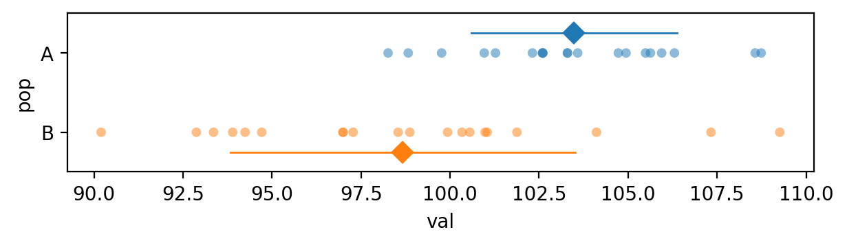
We’ll now apply the Welch’s two-sample t-test to compare the samples from population A and B, which we know are different.
avals = data[data["pop"]=="A"]["val"]
bvals = data[data["pop"]=="B"]["val"]
The sample means seem to reflect the difference between population means too…
avals.mean(), bvals.mean()
(np.float64(103.48610431567451), np.float64(98.67012442302976))
… but we must consider the difference between means relative to the standard deviations of the two samples.
avals.std(), bvals.std()
(np.float64(2.880085264317079), np.float64(4.840193546088457))
Here is a picture that shows the data points, the sample means, and the sample standard deviations for the two samples.
import seaborn as sns

data1 = data[data["pop"].isin(["A","B"])]
with plt.rc_context({"figure.figsize":(7,1.5)}):
    sns.stripplot(data=data1, x="val", y="pop", hue="pop", jitter=0, alpha=0.5)
    sns.pointplot(data=data1, x="val", y="pop", hue="pop", dodge=0.5, estimator="mean",
                  errorbar="sd", marker="D", err_kws={"linewidth":1})
Let’s now use the helper function ttest_dmeans to perform the two-sample t-test calculation
and obtain the \(p\)-value.
from ministats import ttest_dmeans

ttest_dmeans(avals, bvals)
np.float64(0.0005953205918276429)
The \(p\)-value we obtain is 0.000595, which is below the cutoff value \(\alpha=0.05\), so our conclusion is we reject the null hypothesis: the difference between the means of the two unknown populations is statistically significant.
# # ALT.
# from scipy.stats import ttest_ind
# ttest_ind(avals, bvals, equal_var=False)[1]
Effect size#
The confidence interval for the effect size \(\Delta = \mu_A - \mu_B\) is
ci_dmeans(avals, bvals, alpha=0.1, method='a')
[np.float64(2.680529386792265), np.float64(6.95143039849723)]
Example 2: two samples from the same population#
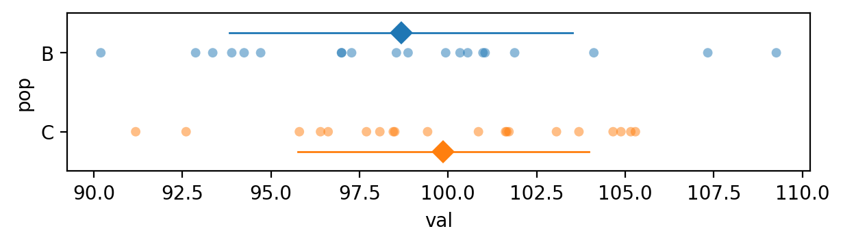
Let’s now analyze the samples from populations B and C that come from the same distribution, which is the situation described by the null hypothesis.
bvals = data[data["pop"]=="B"]["val"]
cvals = data[data["pop"]=="C"]["val"]

bvals.mean(), cvals.mean()
(np.float64(98.67012442302976), np.float64(99.86654813812206))
data2 = data[data["pop"].isin(["B", "C"])]

with plt.rc_context({"figure.figsize":(7,1.5)}):
    sns.stripplot(data=data2, x="val", y="pop", hue="pop", jitter=0, alpha=0.5)
    sns.pointplot(data=data2, x="val", y="pop", hue="pop", dodge=0.5, estimator="mean",
                  errorbar="sd", marker="D", err_kws={"linewidth":1})
from ministats import ttest_dmeans

ttest_dmeans(bvals, cvals)
np.float64(0.40456915642365754)
The \(p\)-value we obtain is 0.40, which is above the cutoff value \(\alpha=0.05\) so our conclusion is that we’ve failed to reject the null hypothesis: the means of two samples are not significantly different.
Effect size#
The confidence interval for the effect size \(\Delta = \mu_B - \mu_C\) is
ci_dmeans(bvals, cvals, alpha=0.1, method='a')
[np.float64(-3.5904215640792363), np.float64(1.1975741338946477)]
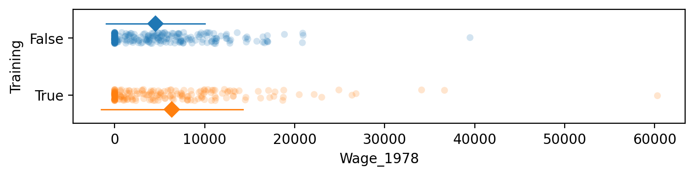
Example 3: Lalonde dataset#
see original paper https://business.baylor.edu/scott_cunningham/teaching/lalonde-1986.pdf
and these links for more info: https://www.one-tab.com/page/h_npVXMeTp2T7Dm5fAlDqw
import pandas as pd
lalonde = pd.read_csv("../datasets/lalonde.csv")
# lalonde.head()
control = lalonde[lalonde["Training"]==False]
treated = lalonde[lalonde["Training"]==True]
# control.describe()
# treated.describe()
# The means of the two groups
treated["Wage_1978"].mean(), control["Wage_1978"].mean()
(np.float64(6349.143530270271), np.float64(4554.801126))
with plt.rc_context({"figure.figsize":(8,1.5)}):
    sns.stripplot(data=lalonde, x="Wage_1978", y="Training", hue="Training",
                  orient="h", alpha=0.2)
    sns.pointplot(data=lalonde, x="Wage_1978", y="Training", hue="Training", dodge=0.5,
                  orient="h", estimator="mean",
                  errorbar="sd", marker="D", err_kws={"linewidth":1})
    plt.legend().remove()
from scipy.stats import ttest_ind

ttest_ind(treated["Wage_1978"], control["Wage_1978"], equal_var=False)
TtestResult(statistic=np.float64(2.674145513783345), pvalue=np.float64(0.00789297771451734), df=np.float64(307.1324931115885))
Effect size#
from ministats import cohend2

cohend2(treated["Wage_1978"], control["Wage_1978"])
np.float64(0.27271540735846483)
Example 4: analysis of a dataset that contains outliers#
The dataset outliers2.csv consists of measurements of “soil score” variable
using a specialized equipment for calculating soil quality.
The measurement apparatus has an upper limit beyound which it doesn’t function properly, so all observations that exceed this limit are recorded as the value 2500.
outliers2 = pd.read_csv("../datasets/outliers2.csv")
outliers2.groupby("group").describe()
| score | ||||||||
|---|---|---|---|---|---|---|---|---|
| count | mean | std | min | 25% | 50% | 75% | max | |
| group | ||||||||
| A | 14.0 | 482.857143 | 681.137833 | 26.0 | 82.50 | 153.5 | 715.75 | 2500.0 |
| B | 18.0 | 1213.611111 | 1099.014486 | 26.0 | 198.75 | 830.0 | 2500.00 | 2500.0 |
with plt.rc_context({"figure.figsize":(7,2)}):
    sns.stripplot(data=outliers2, x="score", y="group", hue="group", jitter=0.2, alpha=0.5)
    sns.pointplot(data=outliers2, x="score", y="group", hue="group", dodge=0.5, estimator="mean",
                  errorbar="sd", marker="D", err_kws={"linewidth":1})
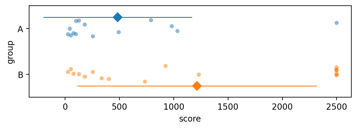
The effect of the outliers in group B is to pull the mean up, to a much higher value than where the other data points are.
from scipy.stats import ttest_ind

scoresA = outliers2[outliers2["group"]=="A"]["score"]
scoresB = outliers2[outliers2["group"]=="B"]["score"]
obst, pvalue = ttest_ind(scoresA, scoresB, equal_var=False)
pvalue
np.float64(0.028387263383781107)
The outliers pull the mean in group B to a high value, which leads us to conclude there is a statistically significant difference between the two groups. This is because we’re using the \(t\)-test when the normality assumption is not valid.
See the example notebook Mann-Whitney_U-test.ipynb for an analysis of this data
using the nonparametric test for comparing two groups,
which is more appropriate for data with outliers.
Discussion#
Links#
For more details about the Welch’s two-sample t-test, see the notebook
notebooks/35_two_sample_tests.ipynb, which contains a more detailed derivation.See the Section 3.5 exercises notebook: exercises/exercises_35_two_sample_tests.ipynb for practice problems.