Mann-Whitney U-test#
The goal of the Mann-Whitney \(U\)-test to compare the medians two unknown population.
This is the nonparametric counterpart of the two-sample \(t\)-test.
import matplotlib.pyplot as plt
import numpy as np
import seaborn as sns
import pandas as pd
%matplotlib inline
%config InlineBackend.figure_format = 'retina'
\(\def\stderr#1{\mathbf{se}_{#1}}\) \(\def\stderrhat#1{\hat{\mathbf{se}}_{#1}}\) \(\newcommand{\Mean}{\textbf{Mean}}\) \(\newcommand{\Var}{\textbf{Var}}\) \(\newcommand{\Std}{\textbf{Std}}\) \(\newcommand{\Freq}{\textbf{Freq}}\) \(\newcommand{\RelFreq}{\textbf{RelFreq}}\) \(\newcommand{\DMeans}{\textbf{DMeans}}\) \(\newcommand{\Prop}{\textbf{Prop}}\) \(\newcommand{\DProps}{\textbf{DProps}}\) \(\newcommand{\med}{m}\) \(\newcommand{\Sgn}{\textbf{Sgn}}\) \(\newcommand{\Rank}{\textbf{Rank}}\)
Data#
Two samples of numerical or ordinal observations \(\mathbf{x}=[x_1, x_2, \ldots, x_n]\) and \(\mathbf{y}=[y_1, y_2,\ldots, y_m]\) from independent populations.
Modeling assumptions#
We don’t need to make any assumptions about the unknown populations.
Hypotheses#
We’re testing \(H_0: \med_X = \med_Y\) against \(H_A: \med_X \neq \med_Y\).
Statistical design#
???
Test statistic#
Compute expressions \(U_1 = \sum_{i=1}^n \Rank(x_i) - \frac{n(n+1)}{2}\) and \(U_2 = \sum_{i=1}^m \Rank(y_i) - \frac{m(m+1)}{2}\), where \(n\) and \(m\) are the sample sizes. We then define \(U = \min(U_1, U_2)\).
Sampling distribution#
For small sample sizes, the exact sampling distribution is obtained through a computational procedure. For large samples, \(U\) is approximately normally distributed.
P-value calculation#
from scipy.stats import mannwhitneyu

# ALT.
# from pingouin import mwu
Examples#
Example 1#
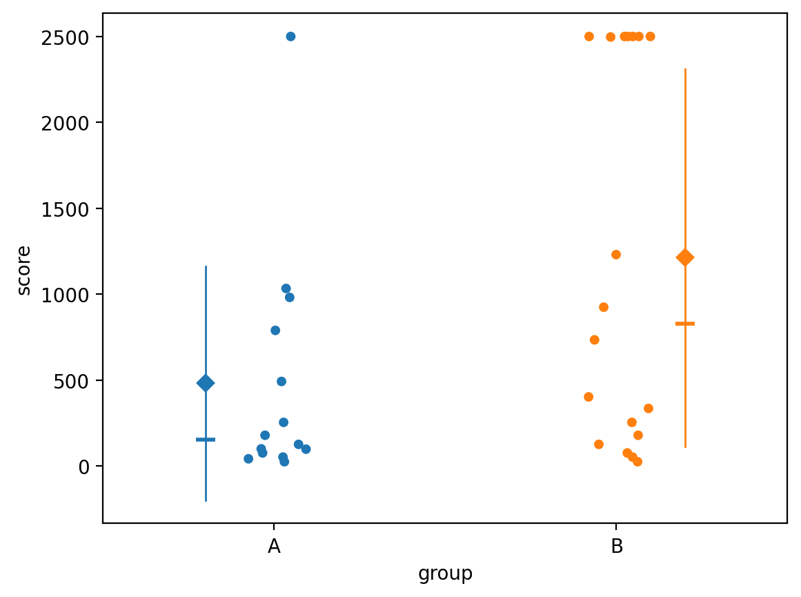
The dataset outliers2.csv consists of measurements of soil score variable
using a specialized equipment for calculating soil quality.
The measurement apparatus has an upper limit beyound which it doesn’t work, so all observations that exceed this limit are coded as the value 2500.
outliers2 = pd.read_csv("../datasets/outliers2.csv")
outliers2.groupby("group").describe()
| score | ||||||||
|---|---|---|---|---|---|---|---|---|
| count | mean | std | min | 25% | 50% | 75% | max | |
| group | ||||||||
| A | 14.0 | 482.857143 | 681.137833 | 26.0 | 82.50 | 153.5 | 715.75 | 2500.0 |
| B | 18.0 | 1213.611111 | 1099.014486 | 26.0 | 198.75 | 830.0 | 2500.00 | 2500.0 |
# plot observations
sns.stripplot(data=outliers2, x="group", y="score", hue="group")

# show means and standard deviations
sns.pointplot(data=outliers2, x="group", y="score", hue="group", dodge=0.4,
              estimator="mean", errorbar="sd", marker="D",
              markersize=5, err_kws={"linewidth":1})

# show also medians
sns.pointplot(data=outliers2, x="group", y="score", hue="group", dodge=0.4,
              estimator="median", errorbar=None, marker="_", markersize=10)
<Axes: xlabel='group', ylabel='score'>
scoresA = outliers2[outliers2["group"]=="A"]["score"]
scoresB = outliers2[outliers2["group"]=="B"]["score"]
Using a regular two-sample t-test#
from scipy.stats import ttest_ind
ttest_ind(scoresA, scoresB, equal_var=False)
TtestResult(statistic=np.float64(-2.3080671633801986), pvalue=np.float64(0.028387263383781107), df=np.float64(28.763605015748688))
The outliers pull the mean in group B to a high value, which leads us to conclude there is a statistically significant difference between the two groups.
Using the Mann-Whitney U-test#
from scipy.stats import mannwhitneyu

mannwhitneyu(scoresA, scoresB)
MannwhitneyuResult(statistic=np.float64(77.0), pvalue=np.float64(0.06389372690752373))
The Mann-Whitney \(U\)-test is better at ignoring the outliers, and correctly fails to reject the null. Indeed, looking at the graph, we see there is not a big difference between the two groups.