Python libraries for doing statistics#
see draft here: https://docs.google.com/document/d/1a-Ohl3hs7w8AiOr85PxW0DZP1ofFK02sk55IEw0zQPE/edit?tab=t.0
Click here to run the notebook interactively, so you can play with the code examples.
Notebook setup#
# Install stats library
%pip install --quiet ministats
[notice] A new release of pip is available: 26.1.1 -> 26.1.2
[notice] To update, run: pip install --upgrade pip
Note: you may need to restart the kernel to use updated packages.
# Figures setup
import matplotlib.pyplot as plt
import seaborn as sns

plt.clf()  # needed otherwise `sns.set_theme` doesn't work
sns.set_theme(
    style="whitegrid",
    rc={'figure.figsize': (7, 2)},
)
# High-resolution figures please
%config InlineBackend.figure_format = 'retina'

def savefig(fig, filename):
    fig.tight_layout()
    fig.savefig(filename, dpi=300, bbox_inches="tight", pad_inches=0)
<Figure size 640x480 with 0 Axes>
Introduction#
IQ scores sample#
Consider the following dataset, which consists of IQ scores of 30 students who took a “smart drug” ☕. The IQ scores are recorded in the following list.
iqs = [ 95.7, 100.1,  95.3, 100.7, 123.5, 119.4,  84.4, 109.6,
       108.7,  84.7, 111.0,  92.1, 138.4, 105.2,  97.5, 115.9,
       104.4, 105.6, 104.8, 110.8,  93.8, 106.6,  71.3, 130.6,
       125.7, 130.2, 101.2, 109.0, 103.8,  96.7]
# data

treated = [92.69, 117.15, 124.79, 100.57, 104.27, 121.56, 104.18,
           122.43, 98.85, 104.26, 118.56, 138.98, 101.33, 118.57,
           123.37, 105.9, 121.75, 123.26, 118.58, 80.03, 121.15,
           122.06, 112.31, 108.67, 75.44, 110.27, 115.25, 125.57,
           114.57, 98.09, 91.15, 112.52, 100.12, 115.2, 95.32,
           121.37, 100.09, 113.8, 101.73, 124.9, 87.83, 106.22,
           99.97, 107.51, 83.99, 98.03, 71.91, 109.99, 90.83, 105.48]

controls = [85.1, 84.05, 90.43, 115.92, 97.64, 116.41, 68.88, 110.51,
            125.12, 94.04, 134.86, 85.0, 91.61, 69.95, 94.51, 81.16,
            130.61, 108.93, 123.38, 127.69, 83.36, 76.97, 124.87, 86.36,
            105.71, 93.01, 101.58, 93.58, 106.51, 91.67, 112.93, 88.74,
            114.05, 80.32, 92.91, 85.34, 104.01, 91.47, 109.2, 104.04,
            86.1, 91.52, 98.5, 94.62, 101.27, 107.41, 100.68, 114.94,
            88.8, 121.8]
Statistics procedures as readable code (ministats)#
Generating sampling distributions#
from ministats import gen_sampling_dist

%psource gen_sampling_dist
One-sample t-test for the mean#
from ministats import ttest_mean
%psource ttest_mean
ttest_mean(iqs, mu0=100, alt="greater")
np.float64(0.01792942680682741)
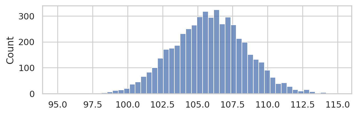
Generating bootstrap distributions#
from ministats import gen_boot_dist

%psource gen_boot_dist
import numpy as np
iqs_boot = gen_boot_dist(iqs, estfunc=np.mean)
sns.histplot(iqs_boot);
The permutation test for comparing two groups#
from ministats.hypothesis_tests import resample_under_H0
from ministats import permutation_test_dmeans

%psource permutation_test_dmeans
%psource resample_under_H0
np.random.seed(43)
permutation_test_dmeans(treated, controls)
0.0098
See the ministats library
for more examples of Python functions that implement the statistical procedures in STATS 101.
In the past, students first contact with statistics was presented as a bunch of procedures without explanation, and students were supposed to memorize when to use which “recipe”. Statistics instructors always had to “skip the details” because it’s super complicated to explain all the details (probability models, sampling distributions, p-value calculations, etc.).
Now that we have Python on our side, we don’t have to water-down the material,
but can instead show all the detailed calculations for statistical tests,
as easy-to-understand Python source code, which makes it much much easier to understand what is going on.
Currently,
the ministats library contains about 400 lines of code.
With a little bit of Python knowledge,
you can read the source code and understand all of statistics.