Descriptive statistics exercises

Descriptive statistics exercises#

This notebook contains all solutions of the exercises from Section 1.3 Descriptive Statistics in the No Bullshit Guide to Statistics.

Notebooks setup#

import numpy as np
import pandas as pd
import matplotlib.pyplot as plt
import seaborn as sns

# Figures setup
sns.set_theme(
    context="paper",
    style="whitegrid",
    palette="colorblind",
    rc={'figure.figsize': (4,2)},
)

%config InlineBackend.figure_format = 'retina'

# Set pandas precision
pd.set_option("display.precision", 2)

# Simple float __repr__
import numpy as np
if int(np.__version__.split(".")[0]) >= 2:
    np.set_printoptions(legacy='1.25')

# Download datasets/ directory if necessary
from ministats import ensure_datasets
ensure_datasets()

datasets/ directory present and ready.

Exercises 1: numerical variables#

E1.16#

Compute the Mean, Min, Max, and Range of the effort variable in the students dataset.

students = pd.read_csv("datasets/students.csv")
efforts = students["effort"]

E1.17#

Find Q1, Med, and Q3 of the effort variable in the students dataset.

E1.18#

Make a one-way frequency table for the effort variable, using \([5,7),\) \([7,9),\) \([9,11),\) \([11,13)\) as the bin intervals.

E1.19#

Consider the following Spear–Tukey box plot of the variable~\(\mathbf{y}\).

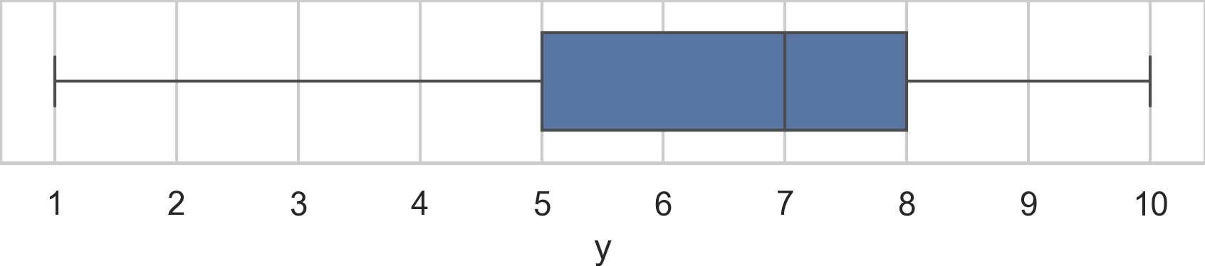
Determine the values of the following descriptive statistics: \(\textbf{med}(\mathbf{y})\), \(\textbf{min}(\mathbf{y})\), \(\textbf{max}(\mathbf{y})\), \(\textbf{Q}_{1}(\mathbf{y})\), \(\textbf{Q}_{2}(\mathbf{y})\), \(\textbf{Q}_{3}(\mathbf{y})\), \(\textbf{IQR}(\mathbf{y})\), and \(\textbf{range}(\mathbf{y})\).

E1.20#

We want to describe the dataset \(\mathbf{x} = (1, 2, 3, 4, 5, 6, 50)\) by reporting a pair of numbers: one measure of central tendency and one measure of dispersion.
a) Compute the mean \(\textbf{mean}(\mathbf{x})\) and the standard deviation \(\textbf{std}(\mathbf{x})\).
b) Compute the median \(\textbf{med}(\mathbf{x})\) and the interquartile range \(\textbf{IQR}(\mathbf{x})\).
c) Which pair of numbers provides a more faithful summary?

xs = pd.Series([1, 2, 3, 4, 5, 6, 50], name="x")

# a) compute the mean and the standard deviation

# b) compute the median and the interquartile range

Exercises 2: two numerical variables#

E1.21#

We’re interested in the age variable and the time variable in the players dataset.

a) Draw a scatter plot of the time versus age
b) Calculate the covariance \(\mathbf{cov}(\texttt{age},\texttt{time})\)
c) Calculate the correlation coefficient \(\mathbf{corr}(\texttt{age},\texttt{time})\)

players = pd.read_csv("datasets/players.csv")

Exercises 3: comparing two groups of numerical variables#

E1.22#

Compare electricity prices between the East and the West parts of the city.

a) generate a strip plot

b) compute the mean for each group

E1.23#

The doctors dataset has the categorical variable loc that represents the location with two possible values rur and urb. Compare the score variable between the rur and urb groups of doctors.

a) scatter plot
b) box plots
c) histograms
d) descriptive statistics

doctors = pd.read_csv("datasets/doctors.csv")

Exercises 4: categorical variables#

E1.24#

Compute frequencies and relative frequencies for the curriculum variable. Display the results in a one-way table.

E1.25#

Make a bar chart displaying the frequencies of the curriculum variable.

E1.26#

What is the mode for variable curriculum in the students dataset? How many times does the modal value occur in the curriculum data?

Exercises 5: two categorical variables#

E1.27#

Given the doctors dataset datasets/doctors.csv, generate:

a) a two-way table of the variables work and loc
b) a grouped bar plot of the variables work and loc
c) a stacked bar plot of the variables work and loc

doctors = pd.read_csv("datasets/doctors.csv")

E1.28#

Load the visitors dataset (datasets/visitors.csv).
a) compute a two-way table of the variables version and bought
b) generate a grouped bar plot of the variables version and bought
c) compute the conditional relative frequencies \(\textbf{relfreq}_{\texttt{1}|\texttt{A}}(\texttt{version}, \texttt{bought})\) and \(\textbf{relfreq}_{\texttt{1}|\texttt{B}}(\texttt{version}, \texttt{bought})\)

visitors = pd.read_csv("datasets/visitors.csv")

# pd.crosstab( ... )

Exercises (end of section)#

E1.29#

Calculate the mean and the standard devoatopm of the variable score variable in the doctors dataset.

E1.30#

A research paper includes these graphs for the variable \(\mathbf{x}\).

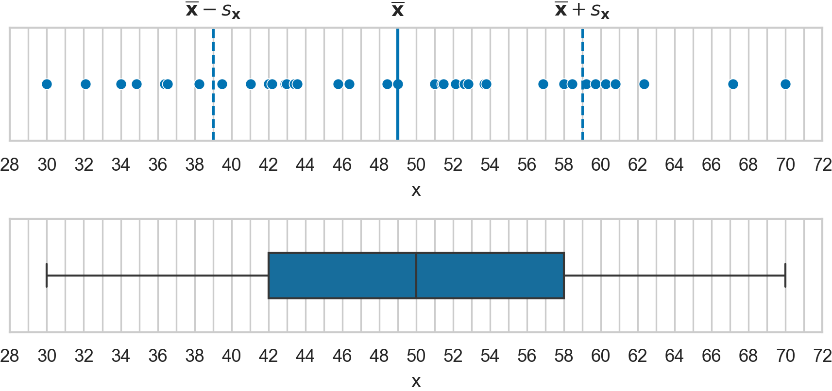
The paper authors forgot to include the numerical summary statistics for the variable \(\mathbf{x}\). Use the information in the graphs to determine the values of the following descriptive statistics: \(\textbf{mean}(\mathbf{x})\), \(\textbf{med}(\mathbf{x})\), \(\textbf{std}(\mathbf{x})\), \(\textbf{var}(\mathbf{x})\), \(\textbf{min}(\mathbf{x})\), \(\textbf{Q}_{1}(\mathbf{x})\), \(\textbf{Q}_{2}(\mathbf{x})\), \(\textbf{Q}_{3}(\mathbf{x})\), \(\textbf{max}(\mathbf{x})\), \(\textbf{IQR}(\mathbf{x})\), \(\textbf{range}(\mathbf{x})\).