Chapter 1 problems

This notebook contains the problems from Chapter 1 Data in the No Bullshit Guide to Statistics.

Notebooks setup

import numpy as np
import pandas as pd
import matplotlib.pyplot as plt
import seaborn as sns

# Figures setup
sns.set_theme(
    context="paper",
    style="whitegrid",
    palette="colorblind",
    rc={"figure.figsize": (5, 2)},
)
%config InlineBackend.figure_format = 'retina'

# Set pandas precision
pd.set_option("display.precision", 2)

# Simple float __repr__
import numpy as np
if int(np.__version__.split(".")[0]) >= 2:
    np.set_printoptions(legacy='1.25')

# Download datasets/ directory if necessary
from ministats import ensure_datasets
ensure_datasets()

Found ../datasets/ and copied files to datasets/.

P1.1

Create a bar plot that compares the mean scores for the debate and lecture groups in the students dataset (datasets/students.csv). The height of each bar should show the mean score for each curriculum type, with error bars indicating the standard deviation for each group.

Hint: Use sns.barplot and set the required value for the errorbar option.

import pandas as pd
students = pd.read_csv("datasets/students.csv")

# bar plot

P1.2

For each of the following sampling scenarios, determine whether the results obtained will apply to the population as a whole.
a) A researcher interested in the mobile usage among 18 year olds used the national citizens registry to obtain a list of all 18 year olds in the country, and randomly selected a sample of size \(n=100\) from this list to contact.
b) A librarian is interested in the lending patterns of digital vs print books for the users of her library. The librarian used the library management system to extract checkout statistics for print books and digital loans for all users of the library for the past five years.
c) The library website administrator ran a survey to collect feedback on the new library discovery tool from the student body. The survey appeared on the website during the month of July and August.
d) A university wants to estimate the proportion of students who have a part-time job, so they ask a random sample of \(n=60\) students from all currently registered students.
e) A researcher wants to estimate the average screen time of teenagers in the country by running a survey on a social media site and analyzing the responses of people who choose to respond.

P1.3

A statistician working for the ministry of health is studying the sleep quality and duration of family doctors in the country. In particular, they are interested in the effectiveness of a new sleep tracking app. For each of the studies described below, determine if it is experimental or observational in nature, and whether it is performed on a representative sample. Will the study results generalize to the population of all doctors in the country? Does the study support a causal conclusion?

a) The researcher uses the national doctors’ registry to select \(100\) doctors at random, and makes them fill out a survey about the number of hours they sleep per night.

b) The researcher places a banner ad on the central web portal that doctors use every day to communicate with their patients. The ad asks doctors to volunteer for a sleep study, and manages to recruit 200 volunteers. The researcher then randomly assigns half of them to use a sleep tracking app and half to a control group that receives some basic educational messaging about the importance of sleep.

c) The researcher selects 200 doctors at random from the national doctors’ registry, and randomly assigns them either to use the sleep tracking app or to the control group (basic educational messaging).

d) The researcher sends a paper survey by mail to all family doctors that asks them about the number of hours they sleep per night, and analyzed the results of the doctors who replied.

P1.4

Classify the following variables according to their level of measurement subtype: nominal, ordinal, interval, or ratio.
a) Body temperature measured in \(^\circ\)C
b) Sleep duration during one night measured in minutes
c) Request priority level (low, medium, high, urgent)
d) File size measured in megabytes
e) Payment method used (cash, credit, debit, e-transfer)
f) T-shirt size (XS, S, M, L, XL, XXL, 3XL)
g) Screen time measured in minutes

P1.5

The data file datasets/markswide.csv contains students’ grades on three tests, and it is organized in “wide” format with columns student_ID, name, test1, test2, test3. Convert this dataset into long format (tidy data) with columns: student_ID, name, test, and grade.

Hint: Use .melt() and set the options id_vars, var_name, and value_name.

import pandas as pd
markswide = pd.read_csv("datasets/markswide.csv")
markswide.head(3)

# use the .melt() method and set the options `id_vars`, `var_name`, and `value_name`

	student_ID	name	test1	test2	test3
0	101	Amelie	74	72	68
1	102	Franklin	62	58	92
2	103	Marge	74	62	83

P1.6

The doctors dataset datasets/doctors.csv contains data from a sleep study. We want to explore the variable score which represents the overall sleep quality score.
a) Generate a strip plot.
b) Generate a box plot.
c) Generate a histogram.
d) Generate a kernel density estimate (KDE) plot.
e) Compute these sample statistics: mean, standard deviation, median, and the quartiles.

import pandas as pd
doctors = pd.read_csv("datasets/doctors.csv")

P1.7

The pandas convenience method .describe() allows us to compute several key descriptive statistics in a single line of code. For example, the code below computes the descriptive statistics for the variable effort from the students dataset.

students = pd.read_csv("datasets/students.csv")
efforts = students["effort"]
efforts.describe()

count    15.00
mean      8.90
std       1.95
min       5.21
25%       7.76
50%       8.69
75%      10.35
max      12.00
Name: effort, dtype: float64

Can you write your own version of the .describe() method from scratch?

# a) Compute count, mean, standard deviaiton, etc. manually

# b) Write a Python function that takes series as input
#    and produces the same output as the `.describe()` method.

def mydescribe(series):
    ...


mydescribe(efforts)

P1.8

Consider the sample \(\mathbf{x} = (10,x_2,x_3)\). Find the values \(x_2\) and \(x_3\) such that \(\overline{\mathbf{x}}=10\) and \(s_{\mathbf{x}}=5\).

P1.9

The dataset \([\mathbf{x}, \mathbf{y}] = [(2,2), (3,3), (4,3), (5,5), (6,4), (5,4), (7,6), (8,5)]\) consists of eight observations of the variables \(x\) and \(y\).
a) Draw a scatter plot of the \((x,y)\) pairs.
b) Compute \(\overline{\mathbf{x}}\), \(s_{\mathbf{x}}\), \(\overline{\mathbf{y}}\), and \(s_{\mathbf{y}}\).
c) Compute the covariance \(\mathbf{cov}(\mathbf{x}, \mathbf{y})\).
d) Compute the correlation coefficient \(\mathbf{corr}(\mathbf{x}, \mathbf{y})\).

Hint: You can use pd.DataFrame([(2,2),(3,3),...],columns=["x","y"]) to create a data frame object from the list of observations.

list_of_obs = [(2,2), (3,3), (4,3), (5,5), (6,4), (5,4), (7,6), (8,5)]

import pandas as pd

P1.10

Consider the following Spear–Tukey box plot of the variable \(\mathbf{z}\).

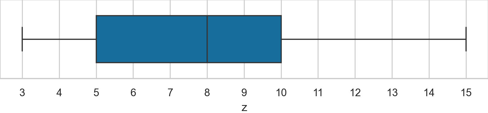
Determine the values of the following descriptive statistics: \(\mathbf{med}(\mathbf{z})\), \(\mathbf{min}(\mathbf{z})\), \(\mathbf{max}(\mathbf{z})\), \(\mathbf{Q}_{1}(\mathbf{z})\), \(\mathbf{Q}_{2}(\mathbf{z})\), \(\mathbf{Q}_{3}(\mathbf{z})\), and \(\mathbf{IQR}(\mathbf{z})\), \(\mathbf{range}(\mathbf{z})\).

P1.11

We want to summarize the dataset \(\mathbf{x}_z = (1, 2, 3, 4, 5, z)\) by reporting a the mean \(\mathbf{mean}(\mathbf{x})\) and the median \(\mathbf{med}(\mathbf{x})\).

import pandas as pd
xs10 = pd.Series([1, 2, 3, 4, 5, 10], name="x")

# a) compute the mean and the median

P1.12

We often encounter non-standard CSV data files. For example, the data file datasets/formats/students_meta.csv contains metadata rows.

# title: Student's dataset with metadata rows
# description: A copy of students.csv with extra metadata at the top
# author: Ivan Savov
# date: 2026-03-25
student_ID,background,curriculum,effort,score
1,arts,debate,10.96,75
2,science,lecture,8.69,75
3,arts,debate,8.6,67
... 12 more lines ...

You’ll get an error if you try loading this file using pd.read_csv with no options. Consult the help docs for the function pd.read_csv to find an option that skips the metadata rows, and load the data below them.

Hint: Use help(pd.read_csv), pd.read_csv?, or the online docs at https://pandas.pydata.org/docs/.

Hint: There are at least two options you can use to skip the metadata rows.

# # This doesn't work:
# students_meta = pd.read_csv("datasets/formats/students_meta.csv")

# Read the `pd.read_csv` help docs and look for options to fix the problem

P1.13

The data file datasets/bpwide.csv is in wide format with columns patient, sex, agegrp, bp_before, and bp_after. The last two columns contain blood pressure measurements taken before and after an intervention. This file is not tidy data since there are two observations per row. Convert the data to tidy data (long format), with the columns patient, sex, agegrp, when, and bp, where the variable when encodes when the measurement was taken (Before or After), and bp contains the corresponding measurement.

import pandas as pd
bpwide = pd.read_csv("datasets/bpwide.csv")
bpwide.head(3)

# Use the .melt() method and set the options `id_vars`, `var_name`, and `value_name`

	patient	sex	agegrp	bp_before	bp_after
0	1	Male	30-45	143	153
1	2	Male	30-45	163	170
2	3	Male	30-45	153	168

P1.14

The data file datasets/kombuchapop.csv contains the volume measurements from all 1000 bottles in the kombucha batches 55 and 56. This is a census of the entire population. We’ll generate a random sample from the batch 55 population to investigate whether random samples really are representative of the population, as we hope they are.
a) Compute the population mean and population standard deviation.
b) Draw a random sample \(\mathbf{k} = \texttt{ksample}\) of size \(n=30\) from the population and compute the sample mean \(\overline{\mathbf{k}}\) and the sample standard deviation \(s_{\mathbf{k}}\).
c) Draw 5000 samples of size \(n=30\) from the population compute the sample mean \(\overline{\mathbf{k}}\) from each of these samples, and plot a histogram of the 5000 sample means \([\overline{\mathbf{k}}_1, \overline{\mathbf{k}}_2, \ldots, \overline{\mathbf{k}}_{5000}]\).
d) Based on the histogram, what can you say about the random sampling approach? Does random sampling produce representative samples?

import pandas as pd
kombuchapop = pd.read_csv("datasets/kombuchapop.csv")
kpopulation = kombuchapop[kombuchapop["batch"]==55]["volume"]

# a) Compute the population mean and standard deviation

# set the random seed to get a reproducible result
np.random.seed(42)

# b) Draw a random sample of size n=30 from `kpopulation`
#    and compute the sample mean and standard deviation.
ksample = ...

# set the random seed to get a reproducible result
np.random.seed(42)

# c) Draw 5000 samples of size n=30 from `kpopulation`,
#    and compute the sample mean from each of these samples
kbars = []
for i in range(5000):
    ksample = ... 
    kbar = ...
    kbars.append(kbar)

# Plot a histogram of the 5000 sample means in `kbars`
# sns.histplot(...)

P1.15

Your friend Ben has written the following function for generating a random sample of size n from a given population.

import numpy as np
from numpy.random import choice

def get_sample(population, n):
    N = len(population)
    nmore, nless = N//2, N - N//2
    ws = np.concat([5*np.ones(nmore), np.ones(nless)])
    p = ws / np.sum(ws)
    sample = choice(population, size=n, replace=False, p=p)
    return sample

Use this function to generate a few samples of size \(n=30\) from Batch 55 of the kombucha population dataset datasets/kombuchapop.csv. Compare the sample means to the population mean. What can you say about the the samples produced by Ben’s sampling function?

import pandas as pd
kombuchapop = pd.read_csv("datasets/kombuchapop.csv")
kpopulation = kombuchapop[kombuchapop["batch"]==55]["volume"]

P1.16

The dataset datasets/howell30.csv contains sex, age, weight, and height information for 298 individuals.

howell30 = pd.read_csv("datasets/howell30.csv")
n = howell30.shape[0]
print("number of individuals:", n)
howell30.head()

number of individuals: 298

	caseid	sex	age	weight	height
0	9	M	27.6	55.5	168.9
1	10	F	19.5	34.9	148.0
2	15	F	21.1	48.4	150.5
3	20	M	13.1	23.2	127.6
4	21	F	8.8	15.8	110.2

Suppose you’re preparing to run a statistical experiment, and you want to randomly assign half the individuals to Group A (the intervention group), and the remaining individuals to Group B (the control group).

a) Write the Python code that performs the random assignment, then compare the average age in the two groups. Did the random assignment produce two groups of equal size? Did the random assignment produce balanced groups with similar average age?

b) Repeat the random assignment procedure 3000 times and calculate the 3000 differences between average age in the two groups. Plot a histogram of the mean age differences. Does random assignment produce balanced groups?

c) Estimate the proportion of the 3000 assignments that led to groups where the average age differs by more than two years. Does the random assignment procedure guarantee the two groups will be balanced?

P1.17

Load the doctors dataset (datasets/doctors.csv) and compute the descriptive statistics for the categorical variables loc and work.
a) The conditional relative frequency \(\mathbf{relfreq}_{\texttt{rur}|\texttt{cli}}(\texttt{loc}, \texttt{work})\).
b) The conditional relative frequency \(\mathbf{relfreq}_{\texttt{cli}|\texttt{rur}}(\texttt{loc}, \texttt{work})\).

Hint: Use the pd.crosstab function with the normalize option.

doctors = pd.read_csv("datasets/doctors.csv")

# a) Conditional relative frequency rur | cli
# pd.crosstab(...)

P1.18

The dataset (datasets/faithful.csv) contains data about the eruptions of the Old Faithful geyser in Yellowstone National Park. We’ll focus on the variable duration, which represents how long each eruption lasted.
a) Compute the mean and the standard deviation of the variable duration.
b) Generate a box plot of the variable duration.
c) Using the information from the previous two answers, what do you think the duration data looks like?
d) Generate a histogram of the variable duration. What does the histogram show that the descriptive statistics didn’t show?

faithful = pd.read_csv("datasets/faithful.csv")
faithful.head(3)

	duration	waiting
0	3.60	79
1	1.80	54
2	3.33	74