
Section 3.5 — Two-sample hypothesis tests#
This notebook contains the code examples from Section 3.5 Two-sample hypothesis tests of the No Bullshit Guide to Statistics.
Notebook setup#
# Ensure required Python modules are installed
%pip install --quiet numpy scipy seaborn pandas ministats
Note: you may need to restart the kernel to use updated packages.
# load Python modules
import os
import numpy as np
import pandas as pd
import seaborn as sns
import matplotlib.pyplot as plt
# Plot helper functions
from ministats import nicebins
from ministats import plot_pdf
from ministats.utils import savefigure

# Stats helper functions
from ministats import tailvalues
from ministats import tailprobs
# Figures setup
plt.clf()  # needed otherwise `sns.set_theme` doesn't work
sns.set_theme(
    context="paper",
    style="whitegrid",
    palette="colorblind",
    rc={"font.family": "serif",
        "font.serif": ["Palatino", "DejaVu Serif", "serif"],
        "figure.figsize": (5, 1.6)},
)
%config InlineBackend.figure_format = 'retina'
<Figure size 640x480 with 0 Axes>
# Simple float __repr__
if int(np.__version__.split(".")[0]) >= 2:
    np.set_printoptions(legacy='1.25')

# set random seed for repeatability
np.random.seed(42)
# Download datasets/ directory if necessary
from ministats import ensure_datasets
ensure_datasets()
datasets/ directory already exists.
\(\def\stderr#1{\mathbf{se}_{#1}}\) \(\def\stderrhat#1{\hat{\mathbf{se}}_{#1}}\) \(\newcommand{\Mean}{\textbf{Mean}}\) \(\newcommand{\Var}{\textbf{Var}}\) \(\newcommand{\Std}{\textbf{Std}}\) \(\newcommand{\Freq}{\textbf{Freq}}\) \(\newcommand{\RelFreq}{\textbf{RelFreq}}\) \(\newcommand{\DMeans}{\textbf{DMeans}}\) \(\newcommand{\Prop}{\textbf{Prop}}\) \(\newcommand{\DProps}{\textbf{DProps}}\)
(this cell contains the macro definitions like \(\stderr{\overline{\mathbf{x}}}\), \(\stderrhat{}\), \(\Mean\), …)
Definitions#
Populations. We’ll label the two unknown populations \(X\) and \(Y\). and assume the arbitrary model family \(\mathcal{M}\) with mean parameter \(X \sim \mathcal{M}(\mu_X)\) and \(Y \sim \mathcal{M}(\mu_Y)\).
Parameters. The means of the two populations \(\mu_X\) and \(\mu_Y\) are unknown, and what we want to study…
Samples. We assume the two samples \(\mathbf{x} = (x_1, x_2, \ldots, x_n)\) and \(\mathbf{y} = (y_1, y_2, \ldots, y_m)\) are randomly selected from the populations \(X\) and \(Y\).
Estimate (statistic) \(\hat{d} = \overline{\mathbf{x}} - \overline{\mathbf{y}}\): the difference between means of the two samples \(\mathbf{x}\) and \(\mathbf{y}\).
Estimator \(\DMeans\): the function that computes the difference between means from two samples, \(\hat{d} = \DMeans(\mathbf{x},\mathbf{y}) = \overline{\mathbf{x}} - \overline{\mathbf{y}}\). the function we use to compute the estimate \(\hat{d}\).
Sampling distribution \(\hat{D} = \DMeans(\mathbf{X}, \mathbf{Y})\): the difference between means computed from two random samples \(\mathbf{X}\) and \(\mathbf{Y}\).
def mean(sample):
    return sum(sample) / len(sample)

def var(sample):
    xbar = mean(sample)
    sumsqdevs = sum([(xi-xbar)**2 for xi in sample])
    return sumsqdevs / (len(sample)-1)

def std(sample):
    s2 = var(sample)
    return np.sqrt(s2)

def dmeans(xsample, ysample):
    dhat = np.mean(xsample) - np.mean(ysample)
    return dhat
Comparing two groups#
Description of the problem: compare two group based on sample means computed from each group.
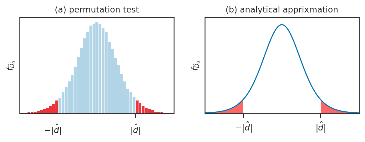
Computing \(p\)-values#
from ministats.book.figures import plot_panel_pvalue_D0_hist_and_dist

fig = plot_panel_pvalue_D0_hist_and_dist();
Simulation examples#
# Two populations X ~ N(120,13) and Y ~ N(100,17)
from scipy.stats import norm
muX, muY = 120, 100
sigmaX, sigmaY = 13, 17
rvX = norm(muX, sigmaX)
rvY = norm(muY, sigmaY)

# Two samples of sizes n=12 and m=15
np.random.seed(49)
n = 12
xsample = rvX.rvs(n)

np.random.seed(53)
m = 15
ysample = rvY.rvs(m)
bins = range(80,140,5)
# sns.histplot(xsample, bins=bins, alpha=0.3)
# sns.histplot(ysample, bins=bins, alpha=0.3)
sns.kdeplot(xsample, bw_adjust=0.3)
sns.kdeplot(ysample, bw_adjust=0.3)
<Axes: ylabel='Density'>
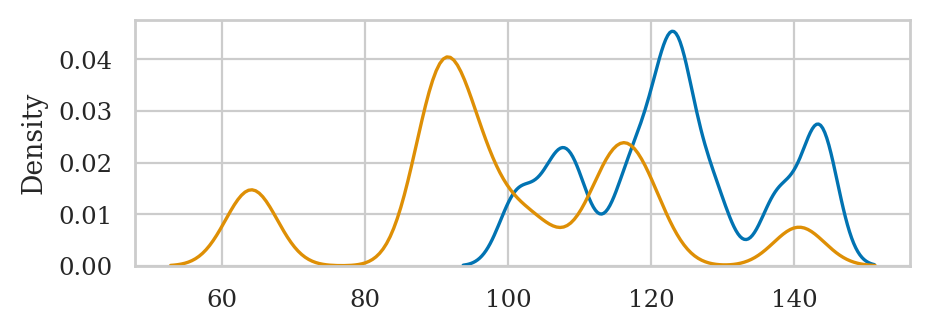
mean(xsample), std(xsample), mean(ysample), std(ysample)
(123.12782102038774, 13.761594639978442, 98.93506558107863, 20.322124432018075)
dmeans(xsample, ysample)
24.19275543930911
3.5.1 Difference between means estimator#
We’ll now discuss an estimators that is specific for the comparison of the two groups.
estimator: \(\hat{d} = \DMeans(\mathbf{x}_A, \mathbf{x}_B) = \Mean(\mathbf{x}_A) - \Mean(\mathbf{x}_B) = \overline{\mathbf{x}}_A - \overline{\mathbf{x}}_B\)
gives an estimate for the difference between population means: \(\Delta = \mu_A - \mu_B\)
def dmeans(xsample, ysample):
    """
    Compute the difference between group means of the samples.
    """
    dhat = np.mean(xsample) - np.mean(ysample)
    return dhat
Example 3: comparison of electricity prices#
Let’s compute the difference between means of the East and West electricity prices.
eprices = pd.read_csv("datasets/eprices.csv")
# eprices
epricesW = eprices[eprices["loc"]=="West"]
pricesW = epricesW["price"]
pricesW
9     11.8
10    10.0
11    11.0
12     8.6
13     8.3
14     9.4
15     8.0
16     6.8
17     8.5
Name: price, dtype: float64
mean(pricesW)
9.155555555555557
var(pricesW)
2.440277777777778
epricesE = eprices[eprices["loc"]=="East"]
pricesE = epricesE["price"]
pricesE
0    7.7
1    5.9
2    7.0
3    4.8
4    6.3
5    6.3
6    5.5
7    5.4
8    6.5
Name: price, dtype: float64
mean(pricesE)
6.155555555555555
var(pricesE)
0.7702777777777778
Let’s calculate the mean of the prices in the East and the West:
mean(pricesW), mean(pricesE)
(9.155555555555557, 6.155555555555555)
To calculate the difference between means,
we can simply subtract these two numbers \(\hat{d} = \overline{\mathbf{x}}_W - \overline{\mathbf{x}}_E\),
or simply call the function dmeans
which computes the estimate \(\hat{d} = \textbf{DMeans}(\tt{pricesW}, \tt{pricesE})\).
dmeans(pricesW, pricesE)
3.000000000000001
According to this estimate, the average price Rob can expect in the East end is three cents cheaper, on average, as compared to the average electricity price in the West.
Sampling distribution of the difference between means#
We assume the two groups are normally distributed random variables \(X\) and \(Y\):
Definitions:
\(\mathbf{x} = (x_1, x_2, \ldots, x_{n})\)=
xsample: a sample of size \(n\) from \(X\)\(\mathbf{y} = (y_1, y_2, \ldots, y_{m})\)=
ysample: a sample of size \(m\) from \(Y\).\(\overline{\mathbf{x}} = \Mean(\mathbf{x})\): the observed mean in the first group
\(\overline{\mathbf{y}} = \Mean(\mathbf{y})\): the observed mean in the second group
\(s_{\mathbf{x}}^2 = \Var(\mathbf{x})\): the sample variance from the first group
\(s_{\mathbf{y}}^2 = \Var(\mathbf{y})\): the sample variance from the second group
\(\hat{d} = \DMeans(\mathbf{x}, \mathbf{y}) = \overline{\mathbf{x}} - \overline{\mathbf{y}}\): the difference between means estimate, which is an estimate of the true different between population means \(\Delta = \mu_X - \mu_Y\).
The sampling distribution of the estimator dmeans is defined as:
where \(\mathbf{X} = (X_1, X_2, \ldots, X_{n})\) and \(\mathbf{Y} = (Y_1, Y_2, \ldots, Y_{m})\) are random samples.
Analytical formula for the sampling distribution#
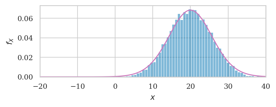
Let’s now use probability theory to build a theoretical model for the sampling distribution of the difference-between-means estimator dmeans.
The central limit theorem tells us the sample mean within the two group are
\[ \overline{\mathbf{X}} \sim \mathcal{N}\!\left(\mu_X, \tfrac{\sigma_X}{\sqrt{n}} \right) \qquad \textrm{and} \qquad \overline{\mathbf{Y}} \sim \mathcal{N}\!\left(\mu_Y, \tfrac{\sigma_Y}{\sqrt{m}} \right). \]The rules of probability theory tells us that the difference of two normal random variables requires subtracting their means and adding their variance, so we get: $\( \hat{D} \sim \mathcal{N}\!\left( \mu_X - \mu_Y, \; \stderr{\hat{D}} \right), \)$
where the standard error of the estimator \(\hat{D}\) is:
\[ \stderr{\hat{D}} = \sqrt{ \tfrac{\sigma^2_X}{n} + \tfrac{\sigma^2_Y}{m} }. \]
Approximation using Student’s \(t\)-distribution#
Recall the plug-in principle allows us to obtain approximate statistical formulas by replacing population parameters with estimates computed from samples. Applying the plug-in principle to the formula \(\stderr{\hat{d}}\), we obtain a formula for the estimated standard error of the difference between means estimator: $\( \stderrhat{\hat{d}} = \sqrt{ \frac{s_{\mathbf{x}}^2}{n} + \frac{s_{\mathbf{y}}^2}{m} } = \sqrt{ \stderrhat{\overline{\mathbf{x}}}^2 + \stderrhat{\overline{\mathbf{y}}}^2 }\;. \)$
We can now build a model for the sampling distribution of the difference between means estimator based on Student’s \(t\)-distribution:
where \(\mathcal{T}(\nu_d)\) is Student’s \(t\)-distribution with \(\nu_d\) degrees of freedom.
The degrees of freedom of is obtained by the following formula $\( \nu_d \;\; = \;\; \frac{ (\stderrhat{\overline{\mathbf{x}}}^2 + \stderrhat{\overline{\mathbf{y}}}^2)^2 } { \frac{\stderrhat{\overline{\mathbf{x}}}^4}{n-1} + \frac{\stderrhat{\overline{\mathbf{y}}}^4}{m-1} }\;. \)$
Let’s write a Python function that calculates the degrees of freedom parameter.
def calcdf(stdX, n, stdY, m):
    vX = stdX**2 / n
    vY = stdY**2 / m
    df = (vX + vY)**2 / (vX**2/(n-1) + vY**2/(m-1))
    return df

# ALT.
# from ministats import calcdf
Example 7: difference between electricity prices#
Let’s return to Bob’s dataset of electricity prices collected from charging stations in the East and West parts of his city. We’ll assume the prices in the two parts of the city are normally distributed and described by the models \(X_W \sim \mathcal{N}(\mu_W, \sigma_W)\) and \(X_E \sim \mathcal{N}(\mu_E, \sigma_E)\).
We have two samples \(\tt{pricesW} = \mathbf{x}_W\) and \(\tt{pricesE} = \mathbf{x}_E\) from these prices
eprices = pd.read_csv("datasets/eprices.csv")
pricesW = eprices[eprices["loc"]=="West"]["price"]
pricesE = eprices[eprices["loc"]=="East"]["price"]
mean(pricesW), mean(pricesE)
(9.155555555555557, 6.155555555555555)
dhat = dmeans(pricesW, pricesE)
dhat
3.000000000000001
# std and sample size in the East
stdW, nW = pricesW.std(), len(pricesW)

# std and sample size in the West
stdE, nE = pricesE.std(), len(pricesE)

stdW, nW, stdE, nE
(1.5621388471508475, 9, 0.8776547030454391, 9)
seD = np.sqrt(stdW**2/nW + stdE**2/nE)
seD
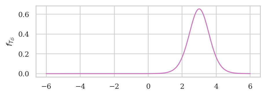
0.5972674401486562
dfD = calcdf(stdW, nW, stdE, nE)
dfD
12.59281702723103
from scipy.stats import t as tdist
rvTDhat = tdist(df=dfD, loc=dhat, scale=seD)
ax = plot_pdf(rvTDhat, rv_name="D", xlims=[-6,6], color="m")
ax.set_ylabel(r"$f_{T_{\widehat{D}}}$")
ax.set_xlabel(None);
Bootstrapped sampling distribution of the difference between means#
First compute bootstrap estimates for mean in each group
from ministats import gen_boot_dist
xbarsW_boot = gen_boot_dist(pricesW, estfunc=mean)
xbarsE_boot = gen_boot_dist(pricesE, estfunc=mean)
Next we compute the difference between means from bootstrap samples
dhats_boot = np.subtract(xbarsW_boot, xbarsE_boot)

ax = sns.histplot(dhats_boot, stat="density", bins=30)
ax.set_xlim([-6,6])
# ax.set_xlabel("$\hat{d}$")
ax.set_ylabel(r"$f_{\widehat{D}^*}$");
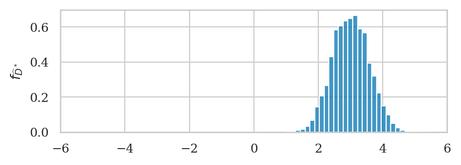
We can obtain the bootstrap estimate of the standard error \(\stderrhat{\hat{d}}^*\) by calculating the standard deviation of the bootstrap distribution.
np.std(dhats_boot)
0.5708757450846252
Note this value is very similar to the value \(\stderrhat{\hat{d}}=0.598\) that we obtained from the analytical approximation formula. This shows that the bootstrap procedure is a viable alternative to the calculation based on analytical approximations.
NEW STUFF (TODO: merge with above)#
TODO: distribute the following plots into appropriate subsections
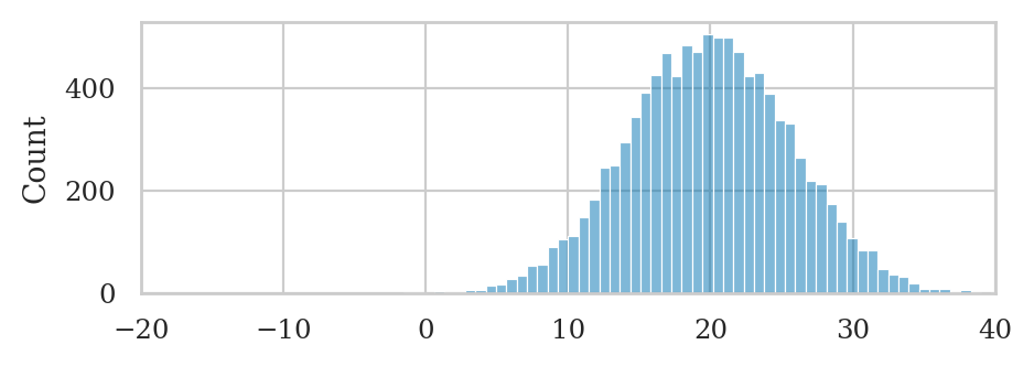
Simulated sampling distribution#
# np.random.seed(42)

N = 10000
dhats = []
for j in range(0,N):
    xsample = rvX.rvs(n)
    ysample = rvY.rvs(m)
    dhat = dmeans(xsample,ysample)
    dhats.append(dhat)

ax = sns.histplot(dhats, alpha=0.5)
ax.set_xlim(-20,40);
Analytical model#
# Standard error
seD = np.sqrt(sigmaX**2/n + sigmaY**2/m)

# Degrees of freedom, the null model, and the t-statistic
from ministats import calcdf
dfD = calcdf(sigmaX, n, sigmaY, m)

# Calculate the p-value from the t-distribution
from scipy.stats import t as tdist
rvD = tdist(df=dfD, loc=muX-muY, scale=seD)
ax = sns.histplot(dhats, stat="density", alpha=0.5)
plot_pdf(rvD, color="C4", ax=ax);
ax.set_xlim(-20,40);
Approximations to the sampling distribution#
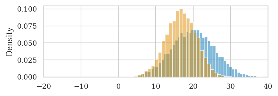
Bootstrap approximation#
from scipy.stats import bootstrap

bres = bootstrap([xsample,ysample], statistic=dmeans, n_resamples=10000)
ax = sns.histplot(dhats, stat="density", alpha=0.5)
sns.histplot(bres.bootstrap_distribution, stat="density", bins=35, color="C1", ax=ax, alpha=0.5);
ax.set_xlim(-20,40);
from ministats import ci_dmeans
ci_dmeans(xsample,ysample, method="b")
[10.094428531239581, 23.256467999865738]
Analytical approximation#
# Estimated standard error
stdX, stdY = std(xsample), std(ysample)
sehatD = np.sqrt(stdX**2/n + stdY**2/m)

# Degrees of freedom, the null model, and the t-statistic
dfD = calcdf(stdX, n, stdY, m)

# Calculate the p-value from the t-distribution
meanX, meanY = mean(xsample), mean(ysample)
print("dhat =", meanX-meanY, "sehatD =", sehatD, "seD", seD)
rvDhat = tdist(df=dfD, loc=meanX-meanY, scale=sehatD)
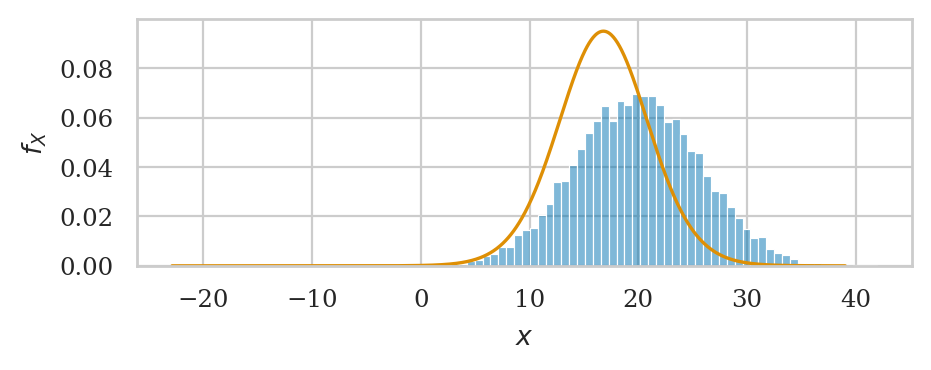
ax = sns.histplot(dhats, stat="density", alpha=0.5)
plot_pdf(rvDhat, color="C1", ax=ax);
dhat = 16.790484536883994 sehatD = 4.149831332963331 seD 5.774945887192364
ci_dmeans(xsample,ysample, method="a")
[9.674487663826724, 23.906481409941293]
Simulated sampling distribution under null#
# Two populations with the same mean X ~ N(100,13) and Y ~ N(100,17)
from scipy.stats import norm
muX0, muY0 = 100, 100
sigmaX0, sigmaY0 = 13, 17
rvX0 = norm(muX0, sigmaX0)
rvY0 = norm(muY0, sigmaY0)

# Two samples of sizes n=12 and m=15
np.random.seed(55)
n = 12
x0sample = rvX0.rvs(n)

np.random.seed(56)
m = 15
y0sample = rvY0.rvs(m)
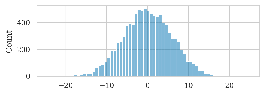
N = 10000
dhats0 = []
for j in range(0,N):
    x0sample = rvX0.rvs(n)
    y0sample = rvY0.rvs(m)
    dhat0 = dmeans(x0sample, y0sample)
    dhats0.append(dhat0)

sns.histplot(dhats0, alpha=0.5);
Sampling distribution from the permutation test#
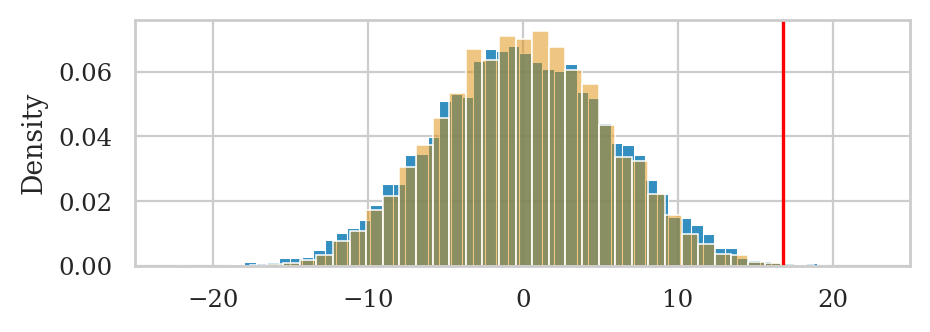
from scipy.stats import permutation_test

np.random.seed(42)
pres = permutation_test([x0sample,y0sample], statistic=dmeans, n_resamples=10000)
ax = sns.histplot(dhats0, stat="density", alpha=0.8)
sns.histplot(pres.null_distribution, stat="density", bins=35, color="C1", ax=ax, alpha=0.5)
plt.axvline(dhat, color="red")
ax.set_xlim(-25,25);
# np.random.seed(45)
from ministats import permutation_test_dmeans
permutation_test_dmeans(xsample, ysample)
0.0005
Sampling distribution from analytical approximation#
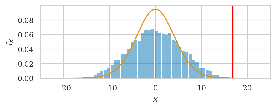
# Estimated standard error
stdX, stdY = std(xsample), std(ysample)
sehatD = np.sqrt(stdX**2/n + stdY**2/m)

# Degrees of freedom, the null model, and the t-statistic
dfD = calcdf(stdX, n, stdY, m)

# Calculate the p-value from the t-distribution
meanX, meanY = mean(xsample), mean(ysample)
rvDhat = tdist(df=dfD, loc=0, scale=sehatD)
ax = sns.histplot(dhats0, stat="density", alpha=0.5)
plot_pdf(rvDhat, color="C1", ax=ax)
plt.axvline(dhat, color="red")
ax.set_xlim(-25,25);
from ministats import ttest_dmeans
ttest_dmeans(xsample, ysample)
0.0005117793326094866
3.5.2 Confidence interval for the difference between means#
Example 3: confidence interval for difference in electricity prices#
eprices = pd.read_csv("datasets/eprices.csv")
pricesW = eprices[eprices["loc"]=="West"]["price"]
pricesE = eprices[eprices["loc"]=="East"]["price"]
The difference between sample means \(\hat{d} = \overline{\mathbf{x}}_W - \overline{\mathbf{x}}_E\) is:
dhat = dmeans(pricesW, pricesE)
dhat
3.000000000000001
The estimate \(\hat{d}\) will be the center of the confidence interval.
Now let’s compute the parameters we need to know to calculate the standard error of the sampling distribution.
# sample size and std in West and East
stdW, nW = pricesW.std(), len(pricesW)
stdE, nE = pricesE.std(), len(pricesE)
stdW, nW, stdE, nE
(1.5621388471508475, 9, 0.8776547030454391, 9)
# standard error
seD = np.sqrt(stdW**2/nW + stdE**2/nE)
seD
0.5972674401486562
# degrees of freedom
from ministats import calcdf

dfD = calcdf(stdW, nW, stdE, nE)
dfD
12.59281702723103
from scipy.stats import t as tdist

# calculate the quantiles of the t-distribution
rvT = tdist(df=dfD)
t_05 = rvT.ppf(0.05)
t_95 = rvT.ppf(0.95)

# construct the confidence interval
[dhat + t_05*seD, dhat + t_95*seD]
[1.9396575883680867, 4.060342411631915]
Bootstrap confidence interval#
# compute bootstrap estimates for mean in each group
np.random.seed(42)
meanW_boot = gen_boot_dist(pricesW, estfunc=mean)
meanE_boot = gen_boot_dist(pricesE, estfunc=mean)

# compute the difference between means of bootstrap samples
dmeans_boot = np.subtract(meanW_boot, meanE_boot)

# construct the confidence interval
[np.percentile(dmeans_boot,5),
 np.percentile(dmeans_boot,95)]
[2.0666666666666664, 3.933888888888892]
Reusable procedure#
def ci_dmeans(xsample, ysample, alpha=0.1, method="a"):
    """
    Compute confidence interval for the difference between population means.
    - method="a" analytical approx. based on Student's t-dist
    - method="b" approx. based on bootstrap estimation
    """
    assert method in ["a", "b"]
    if method == "a":        # analytical approximation
        stdX, n = np.std(xsample, ddof=1), len(xsample)
        stdY, m = np.std(ysample, ddof=1), len(ysample)
        dhat = np.mean(xsample) - np.mean(ysample)
        seD = np.sqrt(stdX**2/n + stdY**2/m)
        dfD = calcdf(stdX, n, stdY, m)
        t_l = tdist(df=dfD).ppf(alpha/2)
        t_u = tdist(df=dfD).ppf(1-alpha/2)
        return [dhat + t_l*seD, dhat + t_u*seD]
    elif method == "b":          # bootstrap estimation
        xbars_boot = gen_boot_dist(xsample, np.mean)
        ybars_boot = gen_boot_dist(ysample, np.mean)
        dmeans_boot = np.subtract(xbars_boot,ybars_boot)
        return [np.quantile(dmeans_boot, alpha/2),
                np.quantile(dmeans_boot, 1-alpha/2)]

# ALT.
# from ministats import ci_dmeans
Verify the coverage probability#
np.random.seed(42)

N = 100  # change to N=1000 for more accuracty
n = 20

from scipy.stats import norm
muX, muY = 120, 100
sigmaX, sigmaY = 10, 10
rvX = norm(muX, sigmaX)
rvY = norm(muY, sigmaY)

acount, bcount = 0, 0
for j in range(0, N):
    xsample = rvX.rvs(n)
    ysample = rvY.rvs(n)
    cia = ci_dmeans(xsample, ysample, alpha=0.1, method="a")
    if cia[0] <= muX - muY <= cia[1]:
        acount += 1
    cib = ci_dmeans(xsample, ysample, alpha=0.1, method="b")
    if cib[0] <= muX - muY <= cib[1]:
        bcount += 1

print("Coverage proportion of analytical approx. CIs:", acount/N)
print("Coverage proportion of bootstrap CIs:", bcount/N)
Coverage proportion of analytical approx. CIs: 0.85
Coverage proportion of bootstrap CIs: 0.84
3.5.3 Permutation test for comparing two populations#
The permutations test is a computational approach for comparing two group. The permutation test takes it’s name from the action of mixing up the group-membership labels and computing a statistic which is a way to generate samples from the null hypothesis in situations where the null hypothesis states there is no difference between two groups.
Permutations#
np.random.seed(43)
np.random.permutation([1,2,3,4,5,6,7])
array([4, 6, 3, 7, 2, 1, 5])
np.random.seed(45)
np.random.permutation([1,2,3,4,5,6,7])
array([6, 3, 2, 1, 5, 7, 4])
Resampling under the null hypothesis#
def resample_under_H0(xsample, ysample):
    """
    Generate new samples from a random permutation of
    the values in the samples `xsample` and `xsample`.
    """
    values = np.concatenate((xsample, ysample))
    pvalues = np.random.permutation(values)
    pxsample = pvalues[0:len(xsample)]
    pysample = pvalues[len(xsample):]
    return pxsample, pysample
# example 1
np.random.seed(43)
resample_under_H0([1,2,3], [4,5,6,7])
(array([4, 6, 3]), array([7, 2, 1, 5]))
# example 2
np.random.seed(45)
resample_under_H0([1,2,3], [4,5,6,7])
(array([6, 3, 2]), array([1, 5, 7, 4]))
The function resample_under_H0 gives us a way to generate samples from the null hypothesis.
We can then compute the value of the dmeans statistic for these samples. We used the assumption of “no difference” under the null hypothesis, and translated this to the “forget the labels” interpretation.
Example 5P: electricity prices#
The probability model under the alternative hypothesis describes two populations with different parameters:
Under the null hypothesis the populations have the same mean:
eprices = pd.read_csv("datasets/eprices.csv")
eprices
| loc | price | |
|---|---|---|
| 0 | East | 7.7 |
| 1 | East | 5.9 |
| 2 | East | 7.0 |
| 3 | East | 4.8 |
| 4 | East | 6.3 |
| 5 | East | 6.3 |
| 6 | East | 5.5 |
| 7 | East | 5.4 |
| 8 | East | 6.5 |
| 9 | West | 11.8 |
| 10 | West | 10.0 |
| 11 | West | 11.0 |
| 12 | West | 8.6 |
| 13 | West | 8.3 |
| 14 | West | 9.4 |
| 15 | West | 8.0 |
| 16 | West | 6.8 |
| 17 | West | 8.5 |
eprices.groupby("loc")["price"].describe()
| count | mean | std | min | 25% | 50% | 75% | max | |
|---|---|---|---|---|---|---|---|---|
| loc | ||||||||
| East | 9.0 | 6.155556 | 0.877655 | 4.8 | 5.5 | 6.3 | 6.5 | 7.7 |
| West | 9.0 | 9.155556 | 1.562139 | 6.8 | 8.3 | 8.6 | 10.0 | 11.8 |
pricesW = eprices[eprices["loc"]=="West"]["price"]
pricesE = eprices[eprices["loc"]=="East"]["price"]

# 1. Calculate the observed difference between means
dprice = dmeans(pricesW, pricesE)
dprice
3.000000000000001
Our goal is to determine how likely or unlikely the observed value \(\hat{d}=3\) is under the null hypothesis \(H_0\). This means we need to obtain the sampling distribution of \(\hat{D}\) under \(H_0\), which we can do using the permutation test.
Let’s look at some of the differences we can expect to observe under \(H_0\).
#######################################################
np.random.seed(31)
# generate new samples by shuffling the labels
ppricesW, ppricesE = resample_under_H0(pricesW, pricesE)

# Compute the difference in means for the bootstrap samples
pdhat0 = dmeans(ppricesW, ppricesE)
pdhat0
1.6444444444444448
Running a permutation test#
We can repeat the resampling procedure 10000 times to get the sampling distribution of \(\widehat{D}_0\) under \(H_0\),
as illustrated in the code procedure below.
np.random.seed(42)

# 2. Obtain the sampling distribution under H0
P = 10000
pdhats0 = []
for i in range(0, P):
    ps1, ps2 = resample_under_H0(pricesW, pricesE)
    pdhat0 = dmeans(ps1, ps2)
    pdhats0.append(pdhat0)
ax = sns.histplot(pdhats0, alpha=0.5)
ax.set_ylabel(r"$f_{\widehat{D}_0}$");
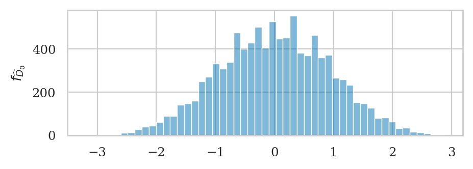
Now that we have the sampling distribution \(\widehat{D}_0\),
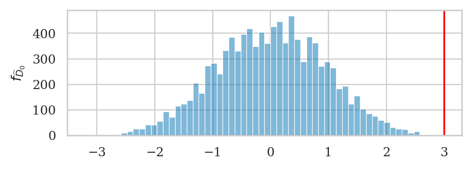
we can see where the observed value \(\hat{d}= 3\) =dprice falls within this distribution.
The \(p\)-value is the probability of observing value dprice=3 or more extreme under the null hypothesis.
# 3. Compute the p-value
tails = tailvalues(pdhats0, dprice, alt="two-sided")
pvalue = len(tails) / len(pdhats0)
pvalue
0.0002
# plot the sampling distribution in blue
bins = nicebins(pdhats0, dprice)
ax = sns.histplot(pdhats0, bins=bins, alpha=0.5)

# plot red line for the observed statistic
plt.axvline(dprice, color="red")

# plot the values that are equal or more extreme in red
sns.histplot(tails, ax=ax, bins=bins, color="red")
ax.set_ylabel(r"$f_{\widehat{D}_0}$");
Effect size estimates#
dprice = dmeans(pricesW, pricesE)
dprice
3.000000000000001
The bootstrap confidence interval for the effect size \(\ci{\Delta,0.9}^*\) tells us a range of plausible values for the effect size.
from ministats import ci_dmeans

np.random.seed(45)
ci_dmeans(pricesW, pricesE, alpha=0.1, method="b")
[2.0777777777777775, 3.9555555555555557]
The 90% confidence interval \(\ci{\Delta,0.9}^* = [2.08, 3.96]\) describes an interval of numbers that should contain the difference between group means \(\Delta\) at least 90% of the time:
Reusable function#
def permutation_test_dmeans(xsample, ysample, P=10000):
    # 1. Compute the observed difference between means
    obsdhat = dmeans(xsample, ysample)

    # 2. Get sampling dist. of `dmeans` under H0
    pdhats0 = []
    for i in range(0, P):
        psx, psy = resample_under_H0(xsample, ysample)
        pdhat0 = dmeans(psx, psy)
        pdhats0.append(pdhat0)

    # 3. Compute the p-value
    tails = tailvalues(pdhats0, obsdhat, alt="two-sided")
    pvalue = len(tails) / len(pdhats0)
    return pvalue
np.random.seed(42)

permutation_test_dmeans(pricesW, pricesE)
0.0002
Example 6P: lecture and debate curriculums#
students = pd.read_csv("datasets/students.csv")
students
| student_ID | background | curriculum | effort | score | |
|---|---|---|---|---|---|
| 0 | 1 | arts | debate | 10.96 | 75.0 |
| 1 | 2 | science | lecture | 8.69 | 75.0 |
| 2 | 3 | arts | debate | 8.60 | 67.0 |
| 3 | 4 | arts | lecture | 7.92 | 70.3 |
| 4 | 5 | science | debate | 9.90 | 76.1 |
| 5 | 6 | business | debate | 10.80 | 79.8 |
| 6 | 7 | science | lecture | 7.81 | 72.7 |
| 7 | 8 | business | lecture | 9.13 | 75.4 |
| 8 | 9 | business | lecture | 5.21 | 57.0 |
| 9 | 10 | science | lecture | 7.71 | 69.0 |
| 10 | 11 | business | debate | 9.82 | 70.4 |
| 11 | 12 | arts | debate | 11.53 | 96.2 |
| 12 | 13 | science | debate | 7.10 | 62.9 |
| 13 | 14 | science | lecture | 6.39 | 57.6 |
| 14 | 15 | arts | debate | 12.00 | 84.3 |
students.groupby("curriculum")["score"].describe()
| count | mean | std | min | 25% | 50% | 75% | max | |
|---|---|---|---|---|---|---|---|---|
| curriculum | ||||||||
| debate | 8.0 | 76.462500 | 10.519633 | 62.9 | 69.55 | 75.55 | 80.925 | 96.2 |
| lecture | 7.0 | 68.142857 | 7.758406 | 57.0 | 63.30 | 70.30 | 73.850 | 75.4 |
studentsD = students[students["curriculum"]=="debate"]
studentsL = students[students["curriculum"]=="lecture"]
scoresD = studentsD["score"]
scoresL = studentsL["score"]

# observed difference between score means
dscore = dmeans(scoresD, scoresL)
dscore
8.319642857142867
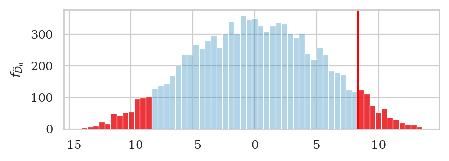
Our goal is to determine how likely or unlikely this observed value \(\hat{d}_s=8.32\) is under the null hypothesis \(H_0\). This means we need to obtain the sampling distribution of \(\hat{D}_0\) under \(H_0\), which we can do using the permutation test.
np.random.seed(43)
pvalue = permutation_test_dmeans(scoresD, scoresL)
pvalue
0.1117
# generate sampling distribution under H0
np.random.seed(43)
pdhats = []
P = 10000
for i in range(0, P):
    rs1, rs2 = resample_under_H0(scoresD, scoresL)
    pdhat = dmeans(rs1, rs2)
    pdhats.append(pdhat)

# plot the sampling distribution in blue
bins = nicebins(pdhats, dscore)
ax = sns.histplot(pdhats, bins=bins, alpha=0.3)

# plot red line for the observed statistic
plt.axvline(dscore, color="red")

# plot the values that are equal or more extreme in red
tails = tailvalues(pdhats, dscore, alt="two-sided")
# print( len(tails) / len(pdhats) )
sns.histplot(tails, bins=bins, ax=ax, color="red")
ax.set_ylabel(r"$f_{\widehat{D}_0}$");
3.5.4 Analytical approximation methods#
We’ll now look at another approach for computing the sampling distribution of the difference between means estimator, using an analytical approximations based on Student’s \(t\)-distribution. This is called the “two-sample \(t\)-test” and it is procedure most commonly taught approach in STATS 101 courses.
How likely or unlikely is the observed difference \(d=3\) under the null hypothesis \(H_0\)?
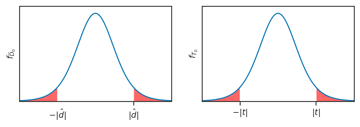
Analytical approximations are math models for describing the sampling distribution under \(H_0\)
Real sampling distributions: obtained by repeated sampling from \(H_0\)
Analytical approximation: math model based on estimated parameters
Based on this assumption we can use the theoretical model for the difference between group means (we assumed the two unknown populations are normally distributed), we can obtain a closed form expression for the sampling distribution of \(D_0\).
In particular, the probability model for the two groups under \(H_0\) are:
\[ H_0: \qquad X = \mathcal{N}({\color{red}{\mu_0}}, \sigma_X) \quad \textrm{and} \quad Y = \mathcal{N}({\color{red}{\mu_0}}, \sigma_Y), \quad \]from which we can derive the model for \(D = \overline{\mathbf{X}} - \overline{\mathbf{Y}}\):
\[ D_0 \sim \mathcal{N}\!\left( {\color{red}{0}}, \; \stderr{\hat{d}} \right) \]In words, the sampling distribution of the difference between group means is normally distributed with mean \(\Delta = 0\) and standard deviation \(\stderrhat{\hat{d}}\), described by the formula:
\[ \stderr{\hat{d}} % \; = \; \sqrt{ \stderr{\overline{\mathbf{x}}}^2 + \stderr{\overline{\mathbf{y}}}^2 } = \sqrt{ \tfrac{\sigma_X^2}{n} + \tfrac{\sigma_Y^2}{m} }\;. \]The standard error of the difference between means depends on the variance of the two groups \(\sigma_X^2\) and \(\sigma_Y^2\). Recall we’ve seen this expression earlier in Section 3.1 and Section 3.2 as well.
Problem 1: the population variances \(\sigma_X^2\) and \(\sigma_Y^2\) are unknown, and we only have the estimated variances \(s_{\mathbf{x}}\) and \(s_{\mathbf{y}}\), which we calculated from the samples \(\mathbf{x}\) and \(\mathbf{y}\).
Solution 1: use plug in estimate and We can obtain an approximation to the standard error of the difference between means estimator using the plug-in principle, which states we can use search-and-replace the population parameters \(\sigma_X^2\) and \(\sigma_Y^2\) with the estimates \(s_{\mathbf{x}}\) and \(s_{\mathbf{y}}\):
\[ \stderrhat{\hat{d}} % \; = \; \sqrt{ \stderrhat{\overline{\mathbf{x}}}^2 + \stderrhat{\overline{\mathbf{y}}}^2 } = \sqrt{ \tfrac{s_{\mathbf{x}}^2}{n} + \tfrac{s_{\mathbf{y}}^2}{m} }\;. \]Problem 2: the estimated standard error \(\stderrhat{\hat{d}}\) tends to underestimate the true standard error \(\stderr{\hat{d}}\), so when we use the basic normal model \(\mathcal{N}\!\left(\tt{loc}=0, \tt{scale}=\stderrhat{\hat{d}} \right)\) the approximation is off (not enough weight in the tails).
Solution 2: use Student’s \(t\)-distribution. We can define a new model for the \(D_0 = \overline{\mathbf{X}} - \overline{\mathbf{Y}}\) based on Student’s \(t\)-distribution: $\( D_0 \sim \mathcal{T}\!\left(\tt{df}=\nu_d, \; \tt{loc}={\color{red}{0}}, \; \tt{scale}=\stderrhat{\hat{d}} \right) \)\( In words, the sampling distribution of the difference between group means can be modeled as Student's \)t\(-distribution with \)\nu_d\( degrees of freedom, centered at \)0\(, with scale parameter \)\stderrhat{\hat{d}}$.
The degrees of freedom parameter, denoted \(\nu_d\) (Greek letter nu) in equations (
dfin code) determines the “weight” in the tails of the distribution. It is computed by a complicated formula that depends on the sample sizes \(n\) and \(m\), and the sample standard deviations \(s_{\mathbf{x}}\) and \(s_{\mathbf{y}}\).
from ministats.book.figures import plot_panel_pvalue_D0_and_T0
plot_panel_pvalue_D0_and_T0();
Example 5T: comparing East and West electricity prices#
eprices = pd.read_csv("datasets/eprices.csv")
pricesW = eprices[eprices["loc"]=="West"]["price"]
pricesE = eprices[eprices["loc"]=="East"]["price"]

# Calculate the observed difference between means
dprice = dmeans(pricesW, pricesE)
dprice
3.000000000000001
Two-sample t-test#
We’ll now show the data, probability modeling, and calculation steps of the “two-sample \(t\)-test for comparing group means. The two-sample \(t\)-test is also known as Welch’s t-test.
# Calculate the sample size and the standard deviation for each group
nW, nE = len(pricesW), len(pricesE)
stdW, stdE = std(pricesW), std(pricesE)
# Compute the standard error of the estimator D
seD = np.sqrt(stdW**2/nW + stdE**2/nE)
seD
0.5972674401486561
# Compute the value of the t-statistic
obst = (dprice - 0) / seD
obst
5.022875513276465
from ministats import calcdf

# Obtain the degrees of freedom from the crazy formula
dfD = calcdf(stdW, nW, stdE, nE)
dfD
12.59281702723103
# Calculate the p-value

from scipy.stats import t as tdist
rvT0 = tdist(df=dfD)
from ministats import tailprobs
pvalue = tailprobs(rvT0, obst, alt="two-sided")
pvalue
0.0002570338337217684
# # SKIP BECAUSE TOO SMALL TO SEE
# _, ax = calc_prob_and_plot_tails(rvT0, -obst, obst, xlims=[-6,6])
# ax.set_title(None)
# ax.set_xlabel("$t$")
# ax.set_ylabel("$f_{T_0}$");
Effect size estimates#
dprice = dmeans(pricesW, pricesE)
dprice
3.000000000000001
The confidence interval for the effect size \(\ci{\Delta,0.9}\) tells us a range of plausible values for the effect size.
from ministats import ci_dmeans

ci_dmeans(pricesW, pricesE, alpha=0.1, method="a")
[1.9396575883680867, 4.060342411631915]
The 90% confidence interval \(\ci{\Delta,0.9} = [1.94, 4.06]\) describes an interval of numbers that should contain the difference between group means \(\Delta\) at least 90% of the time:
Reusable procedure for two-sample \(t\)-test#
def ttest_dmeans(xsample, ysample):
    # Calculate the observed difference between means
    obsdhat = mean(xsample) - mean(ysample)

    # Calculate the sample sizes and the stds
    n, m = len(xsample), len(ysample)
    sx, sy = std(xsample), std(ysample)

    # Calculate the standard error, the degrees of
    # freedom, the null model, and the t-statistic
    seD = np.sqrt(sx**2/n + sy**2/m)
    dfD = calcdf(sx, n, sy, m)
    obst = (obsdhat - 0) / seD

    # Calculate the p-value from the t-distribution
    rvT0 = tdist(df=dfD)
    pvalue = tailprobs(rvT0, obst, alt="two-sided")
    return pvalue
Verify we get the same \(p\)-value when using the standard error formula.
ttest_dmeans(pricesW, pricesE)
0.0002570338337217683
Example 6T: comparing rural and urban sleep scores#
students = pd.read_csv("datasets/students.csv")
# students
# students.groupby("curriculum")["score"].describe()

scoresD = students[students["curriculum"]=="debate"]["score"]
scoresL = students[students["curriculum"]=="lecture"]["score"]

# observed difference between score means
dscores = dmeans(scoresD, scoresL)
dscores
8.319642857142867
ttest_dmeans(scoresD, scoresL)
0.10307495448387385
# T-TEST ANALYSIS
nD, nL = len(scoresD), len(scoresL)
stdD, stdL = std(scoresD), std(scoresL)
seDDL = np.sqrt(stdD**2/nD + stdL**2/nL)

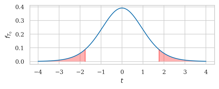
obstDL = (dscores - 0) / seDDL

from ministats import calcdf
dfDL = calcdf(stdD, nD, stdL, nL)
rvT0DL = tdist(df=dfDL)
pvalueDL = tailprobs(rvT0DL, obstDL, alt="two-sided")
pvalueDL
0.10307495448387385
from ministats import calc_prob_and_plot_tails
_, ax = calc_prob_and_plot_tails(rvT0DL, -obstDL, obstDL, xlims=[-4,4])
ax.set_title(None)
ax.set_xlabel("$t$")
ax.set_ylabel("$f_{T_0}$");
Alternative calculation methods#
Two-sample \(t\)-test using pooled variance#
Pooled variance formulas#
Example 5T revisited with pooled variance#
# TODO make self contained
# Compute the pooled variance and standard error of estimator D
varp = ((nW-1)*stdW**2 + (nE-1)*stdE**2) / (nW + nE - 2)
stdp = np.sqrt(varp)
seDp = stdp * np.sqrt(1/nW + 1/nE)
seDp
0.5972674401486561
# Compute the value of the t-statistic
obstp = (dprice - 0) / seDp
obstp
5.022875513276465
# Obtain the degrees of freedom
dfDp = nW + nE - 2
dfDp
16
from scipy.stats import t as tdist
from ministats import tailprobs

# Calculate the p-value
rvT0p = tdist(df=dfDp)
pvaluep = tailprobs(rvT0p, obstp, alt="two-sided")
pvaluep
0.00012497067987674883
Bootstrap confidence interval using scipy#
# two-sample test `scipy.stats`
from scipy.stats import bootstrap

np.random.seed(42)
res = bootstrap([pricesW, pricesE], statistic=dmeans,
                confidence_level=0.9, n_resamples=5000,
                vectorized=False, method="percentile")
[res.confidence_interval.low,
 res.confidence_interval.high]
[2.0666666666666655, 3.933888888888892]
Note the result is the same as …
Confidence intervals using statsmodels#
import statsmodels.stats.api as sms

statsW = sms.DescrStatsW(pricesW)
statsE = sms.DescrStatsW(pricesE)
cm = sms.CompareMeans(statsW, statsE)
cm.tconfint_diff(alpha=0.1, usevar="unequal")
(1.9396575883680864, 4.060342411631914)
Note the result is the same as …
In the above code example, the functions sms.DescrStatsW compute the descriptive statistics
for the two samples, then sms.CompareMeans performs the comparison of means statistical analysis.
We call the method tconfint_diff to extract the 90% confidence interval from the result.
As you can see,
the numbers we obtain from the statsmodels
is exactly the same as the confidence interval we computed manually.
Confidence interval using pinguouin#
import pingouin as pg

res = pg.ttest(pricesW, pricesE, confidence=0.9, correction=True)
res["CI90"].values[0]
array([1.93965759, 4.06034241])
Using scipy.stats.permutation_test for permutation test#
You can use the SciPy implementation of permutation test,
by calling the function permutation_test to perform a permutation test, then obtain the \(p\)-value.
from scipy.stats import permutation_test

np.random.seed(42)

res3 = permutation_test([pricesW,pricesE], statistic=dmeans, n_resamples=10000)
res3.pvalue
0.00019998000199980003
Note the \(p\)-value we obtained form the two methods may be different. This can happen when using the permutations test, because we use randomness as part of the calculation.
Using scipy.stats.ttest_ind for two-sample \(t\)-tests#
Alternatively,
we can use scipy.stats.ttest_ind to obtain the \(p\)-value.
Use equal_var=False to obtain the Welsh value.
# ALT. compute using existing function in `scipy.stats`
from scipy.stats import ttest_ind
res1 = ttest_ind(pricesW, pricesE, equal_var=False)
res1.pvalue
0.0002570338337217615
Use equal_var=True to obtain the pooled variance value.
# ALT. compute using existing function in `scipy.stats`
from scipy.stats import ttest_ind
res2 = ttest_ind(pricesW, pricesE, equal_var=True)
res2.pvalue
0.00012497067987678512
Using statsmodels for two-sample \(t\)-tests#
import statsmodels.stats.api as sms

statsW = sms.DescrStatsW(pricesW)
statsE = sms.DescrStatsW(pricesE)
cm = sms.CompareMeans(statsW, statsE)

# Welch's t-test
cm.ttest_ind(alternative="two-sided", usevar="unequal")
(5.022875513276463, 0.00025703383372176225, 12.592817027231028)
# T-test with pooled variance
cm.ttest_ind(alternative="two-sided", usevar="pooled")
(5.022875513276463, 0.0001249706798767854, 16.0)
Explanations#
Statistical modelling assumptions#
INDEP:
NORMAL:
LARGEn:
EQVAR:
Standardized effect size#
It is sometimes useful to report the effect size using a “standardized” measure for effect sizes.
Cohen’s \(d\) is one such measure, and it is defined as the difference between two means divided by the pooled standard deviation.
where the pooled variance is defined as \(s_{p}^2 = [(n -1)s_{\mathbf{x}}^2 + (m -1)s_{\mathbf{y}}^2]/(n + m -2)\).
def cohend2(sample1, sample2):
    """
    Cohen's d measure of effect size for two independent samples.
    """
    n1, n2 = len(sample1), len(sample2)
    mean1, mean2 = mean(sample1), mean(sample2)
    var1, var2 = var(sample1), var(sample2)
    # calculate the pooled variance and std
    var_pooled = ((n1-1)*var1+(n2-1)*var2) / (n1+n2-2)
    std_pooled = np.sqrt(var_pooled)
    d = (mean1 - mean2) / std_pooled
    return d
We interpret the value of Cohen’s \(d\) using the reference table of values:
Cohen’s d |
Effect size |
|---|---|
0.01 |
very small |
0.20 |
small |
0.50 |
medium |
0.80 |
large |
Effect size for mean deviation of kombucha Batch 04 from expected value \(\mu_K=1000\).
cohend2(pricesW, pricesE)
2.3678062243290996
Discussion#
Comparison to resampling methods#
Exercises#
See notebook sec35_comparing_two_groups.ipynb.
Links#

CUT MATERIAL#
Example sampling dist using pivotal transformation#
Recall the sampling distribution of the difference between means rvTDhat.
Here are some examples of equivalent calculations using standard \(t\)-distribution.
dfD = calcdf(stdW, nW, stdE, nE)
rvT = tdist(df=dfD)
rvTDhat.ppf(0.95), rvT.ppf(0.95)*seD + dhat
(4.060342411631915, 4.060342411631915)
rvTDhat.cdf(4), rvT.cdf( (4-dhat)/seD )
(0.9406438830093703, 0.9406438830093703)